Worksheet 8-2: Orthogonal Projection (with Solutions)

Download: CMSE382-WS8_2.pdf, CMSE382-WS8_2-Soln.pdf

Warning

This is an AI-generated transcript of the worksheet and may contain errors or inaccuracies. Please refer to the original course materials for authoritative content.

---

Worksheet 8-2: Q1

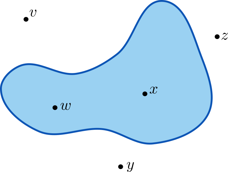
For the following sets and each point drawn (\(v\), \(w\), \(x\), \(y\), and \(z\)), mark the point that minimizes the projection operator (\(P_C(v)\), \(P_C(w)\), \(P_C(x)\), \(P_C(y)\), and \(P_C(z)\)).

Solution

---

Worksheet 8-2: Q2

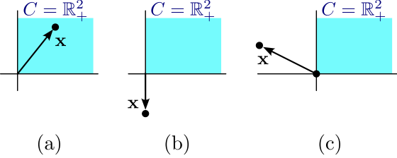
For each of the shown vectors \(\mathbf{x}\), answer the following

1. Find an expression for the non-negative real part \([\mathbf{x}]_+\) in terms of \(\mathbf{x} = (x_1,x_2)\).

Solution

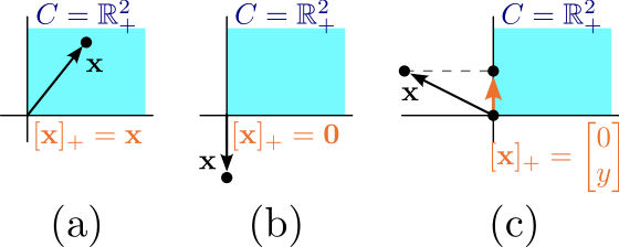
(a) The point is already in the non-negative orthant, so \([\mathbf{x}]_+ = \mathbf{x}\).

(b) The point is in the negative orthant, so \([\mathbf{x}]_+ = \mathbf{0}\).

(c) \(x_1\) is negative and \(x_2\) is positive, so \([\mathbf{x}]_+ = (0,x_2)\).

1. Sketch \([\mathbf{x}]_+\) for each vector.

Solution

---

Worksheet 8-2: Q3

1. Consider the set \(C = \{(y_1,y_2,y_3) \in \mathbb{R}^3 \mid y_1\geq 0, y_2\geq 0, y_3 = 0 \}\). Write the orthogonal projection operator \(P_C(\mathbf{x})\) for any \(\mathbf{x} = (x_1,x_2,x_3) \in \mathbb{R}^3\). What point in \(C\) minimizes \(P_c(\mathbf{x})\)? Write it in terms of \([\cdot]_+\) if possible.

Solution

• The projection operator is \(P_C(\mathbf{x}) = \mathbf{y}\) where \(\mathbf{y}\) minimizes

\[ \min_{\mathbf{y}} \| \mathbf{x} - \mathbf{y}\|^2 \]

• which is equivalent to

\[ \min_{\mathbf{y}} (x_1-y_1)^2 + (x_2-y_2)^2 + (x_3-0)^2. \]

• This is separable, so the projection is the point \((y_1,y_2,y_3)\) that minimizes \((y_1-x_1)^2\), \((y_2-x_2)^2\), and \((x_3)^2\) separately (since \(y_3=0\)).

• This means the point in \(C\) that minimizes both functions is \(P_C(\mathbf{x}) = ([x_1]_+, [x_2]_+, 0)\).

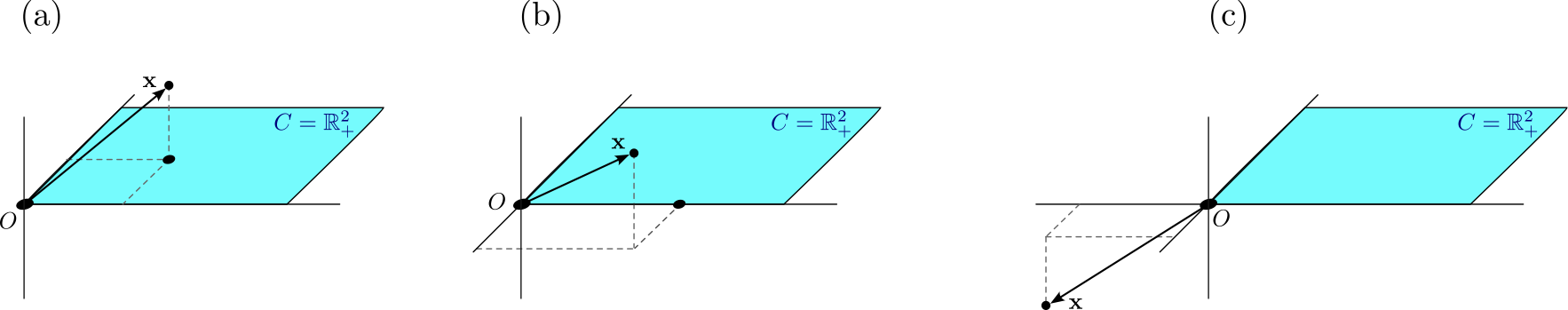
1. For each of the following points, write the expression for the projected point in terms of just \(x_1, x_2, x_3\). Sketch the point.

Solution

(a) Since \(x_1, x_2, x_3 \geq 0\), we have

\[ P_C(\mathbf{x}) = ([x_1]_+, [x_2]_+, 0) = (x_1,x_2,0) \]

(b) Here, \(x_1, x_3 \geq 0\), but \(x_2 \leq 0\). So we have

\[ P_C(\mathbf{x}) = ([x_1]_+, [x_2]_+, 0) = (x_1,0,0) \]

(c) In this case, \(x_1,x_2,x_3 \leq 0\), so

\[ P_C(\mathbf{x}) = ([x_1]_+, [x_2]_+, 0) = (0,0,0) \]

---

Worksheet 8-2: Q4

A box is a subset of \(\mathbb{R}^n\) of the form

\[\begin{split} \begin{align*} B &= [\ell_1,u_1]\times [\ell_2, u_2]\times \ldots \times [\ell_n,u_n]\\ & =\{\mathbf{x} \in \mathbb{R}^n: \ell_i \leq x_i \leq u_i\}, \end{align*} \end{split}\]

where \(\ell_i \leq u_i\) for all \(i=1,2,\ldots,n\).

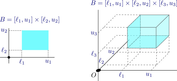
We will assume that some of the \(u_i\)s can be \(\infty\) and some of the \(\ell_i\)s can be \(-\infty\); but in these cases we will assume that \(-\infty\) or \(\infty\) are not contained in the intervals. The figure above shows some two examples in boxes in \(\mathbb{R}^2\) and \(\mathbb{R}^3\). The orthognal projection on the box is the minimizer of the convex optimization problem

\[\begin{split} \begin{aligned} & \text{min} & & \|\mathbf{y}-\mathbf{x}\|^2 \\ & \text{s.t.} & & \mathbf{y} \in B \end{aligned} \end{split}\]

for a given box \(B\).

1. Write the minimization problem above in terms of only \(x_i\)’s and \(y_i\)’s.

Solution

\[\begin{split} \begin{aligned} & \text{min} & & \sum_{i=1}^n (y_i-x_i)^2 \\ & \text{s.t.} & & y_i \in [\ell_i, u_i] \text{ for each }i \end{aligned} \end{split}\]

1. Is the resulting functional equation separable? Justify your answer.

Solution

Yes it’s separable. This is exactly the definition since I have the function in pieces that each only depend on one of the constraints.

1. Write down and solve the optimization problem for each \(y_i\). Use this to determine \(\mathbf{y} = P_C(\mathbf{x})\).

Solution

The problem becomes

\[ \min\{(y_i-x_i)^2 \mid y_i \in [\ell_i,u_i] \} \]

which has value 0 if \(x_i \in [\ell_i,u_i]\) since we just set \(y_i = x_i\). On the other hand, if \(x_i<\ell_i\), the minimum occurs at the lower bound \(y_i = \ell_i\), and similarly if \(x_i>u_i\), it occurs at \(y_i = u_i\). Putting this together, the optimum is at

\[\begin{split} y_i = \begin{cases} u_i, & x_i \geq u_i,\\ x_i, & \ell_i < x_i < u_i,\\ \ell_i & x_i \leq \ell_i, \end{cases} \end{split}\]

and so the full solution is \(\mathbf{y} = (y_1,\cdots,y_n)\) for the \(y_i\)’s given above.

---

Worksheet 8-2: Q5

Consider the normal ball in \( \mathbb{R}^2\), \(C = B[0,r] = \{\mathbf{y} =(y_1,y_2) \mid \|\mathbf{y}\|_2 \leq r\}\). We will find the projection \(P_C(\mathbf{x})\) for some point \(\mathbf{x} \in \mathbb{R}^2\), which is the \(\mathbf{y}\) that minimizes

\[\begin{split} \begin{aligned} & \text{min} & & \|\mathbf{y}-\mathbf{x}\|^2 \\ & \text{s.t.} & & \|\mathbf{y}\|^2 \leq r^2. \end{aligned} \end{split}\]

1. Assume \(\mathbf{x} \in B[0,r]\). What is \(P_C(\mathbf{x})\) and why?

Solution

\(P_C(\mathbf{x}) = \mathbf{x}\) since \(\|x \leq r^2\) as it’s in \(B[0,r]\), so then the function becomes

\[\|\mathbf{y}-\mathbf{x}\|^2 = \|\mathbf{x}-\mathbf{x}\|^2 = 0\]

and this function is always \(\geq 0\), so this must be the minimum.

1. What is \(\nabla f(\mathbf{z})\) for \(f(\mathbf{z}) = \|\mathbf{z}\|^2\)?

Solution

This works for any dimension, but we’re just focused on \( \mathbb{R}^2\) right now. So think of \(f(z_1,z_2) = z_1^2 + z_2^2\) to write the gradient as

\[\begin{split} \nabla f(\mathbf{z}) = \begin{bmatrix} 2z_1 \\ 2z_2 \end{bmatrix} = 2 \begin{bmatrix} z_1 \\ z_2 \end{bmatrix} = 2\mathbf{z} \end{split}\]

1. Now we can deal with the case where \(\mathbf{x} \not\in B[0,r]\), equivalently \(\|\mathbf{x}\|^2 \geq r^2\). We know (from the first order optimality condition for local optima, Thm 2.6 in the book) that if \(\mathbf{x}^* \in \text{int}(C)\) is a local optimum and all partial derivatives exist, then \(\nabla f(\mathbf{x}^*) = 0\). If \(\mathbf{x} \not\in B[0,r]\) and somehow \(\mathbf{x}^* = P_C(\mathbf{x}) \in \text{int}(B[0,r])\), use your calculated gradient above to conclude that the result is impossible so \(P_C(\mathbf{x})\) must be on the boundary of \(B[0,r]\).

Solution

If \(\mathbf{x}^* = P_C(\mathbf{x}) \in \text{int}(B[0,r])\), the theorem mentioned says that we must have \(\nabla f(\mathbf{x}^*) = 0\). But by the calculation above, this is the optimum of \(f(\mathbf{x}-\mathbf{y}) = \|\mathbf{x}-\mathbf{y}\|^2\), so \(\nabla f = 2(\mathbf{x}^* - \mathbf{x}) = \), but then \(\mathbf{x}^* = \mathbf{x}\). The problem is \(\mathbf{x} \not \in B[0,r]\) but \(\mathbf{x}^* \in B[0,r]\), so they can’t be the same point. This means that our assumption that \(\mathbf{x}^*\) was in the interior of \(B[0,r]\) must be wrong, so \(\mathbf{x}^*\) is on the boundary.

1. By the previous, we know that if \(\|\mathbf{x}\|\geq r\), the solution must be on the boundary, so we can replace the problem with

\[\begin{split} \begin{aligned} & \text{min} & & \|\mathbf{y}-\mathbf{x}\|^2 \\ & \text{s.t.} & & \|\mathbf{y}\|^2 = r^2. \end{aligned} \end{split}\]

Then I can expand \(\|\mathbf{y}-\mathbf{x}\|^2 = \|\mathbf{y}\|^2 -2 \mathbf{y}^\top \mathbf{x} + \|\mathbf{x}\|^2\) and replace this problem with

\[\begin{split} \begin{aligned} & \text{min} & & \|\mathbf{y}\|^2 -2 \mathbf{y}^\top \mathbf{x} + \|\mathbf{x}\|^2 \\ & \text{s.t.} & & \|\mathbf{y}\|^2= r^2. \end{aligned} \end{split}\]

Why, then, can I replace this problem with the following problem?

\[\begin{split} \begin{aligned} & \text{min} & & -2 \mathbf{y}^\top \mathbf{x} \\ & \text{s.t.} & & \|\mathbf{y}\|^2 = r^2. \end{aligned} \end{split}\]

Solution

We know that \(\|y\|^2 = r^2\) is a constant that doesn’t depend on \(\mathbf{y}\). Also, \(\|\mathbf{x}\|^2\) doesn’t depend on \(\mathbf{y}\). So \(\|\mathbf{y}\|^2 + \|\mathbf{x}\|^2\) is a constant as far as \(\mathbf{y}\) is concerned. So the optimization will find a minimum at the same \(\mathbf{y}\) whether we use

\[\|\mathbf{y}-\mathbf{x}\|^2 = -2 \mathbf{y}^\top \mathbf{x} + \text{constant}\]

or just \(-2 \mathbf{y}^\top \mathbf{x}\).

1. The Cauchy-Schwartz inequality (\(|\mathbf{u}^\top \mathbf{v}| \leq \|\mathbf{u}\| \cdot \|\mathbf{v}\|\)) gives us a bound

\[ \mathbf{y}^\top \mathbf{x} \leq |\mathbf{y}^\top \mathbf{x}| \leq \|\mathbf{y}\| \cdot \|\mathbf{x}\| \]

Use the above to justify each inequality below.

\[ -2 \mathbf{y}^\top \mathbf{x} \geq -2\|\mathbf{y}\| \|\mathbf{x}\| = -2r\|\mathbf{x}\|. \]

Solution

The first inequality comes from multiplying the top equation by \(-2\) and reversing the inequality because it’s negative. The second equality is because \(\mathbf{y}\) is on the boundary of the ball, so \(\|\mathbf{y}\| = r\).

1. Check that equality in Eqn. (bound) (meaning \(-2 \mathbf{y}^\top \mathbf{x} = -2r\|\mathbf{x}\|\)) occurs when \(\mathbf{y}^* = r\frac{\mathbf{x}}{\|\mathbf{x}\|}\).

Solution

Notice we can just drop the \(-2\) on each side to see if \(\mathbf{y}^\top \mathbf{x} = r\|\mathbf{x}\|\). Plugging in \(\mathbf{y} = \mathbf{y}^*\) on the left gives

\[ \begin{align*} \mathbf{y}^\top \mathbf{x} & = \frac{r}{\|\mathbf{x}\|} \mathbf{x}^\top \mathbf{x} =\frac{r}{\|\mathbf{x}\|}\|\mathbf{x}\|^2 = r\|\mathbf{x}\|. \end{align*} \]

1. Check that \(\mathbf{y}^* = r\frac{\mathbf{x}}{\|\mathbf{x}\|}\) is in \(B[0,r]\).

Solution

In this case, we just need to be sure it is on the boundary, so I need \(\|\mathbf{y}^*\|^2 = r^2\). But we can check this since

\[ \|\mathbf{y}^*\|^2 = \left\|r\frac{\mathbf{x}}{\|\mathbf{x}\|} \right\|^2 = \frac{r^2}{\|\mathbf{x}\|^2} \left\|\mathbf{x} \right\|^2 = r^2 \]

like we wanted.

1. Putting the above together, fill in the orthogonal projection for the ball:

\[\begin{split} P_{B[0,r]} = \begin{cases} \boxed{\phantom{\prod} \phantom{\prod}} & \|\mathbf{x}\|\leq r \\ \\ \boxed{\phantom{\prod} \phantom{\prod}} & \|\mathbf{x}\| > r \end{cases} \end{split}\]

Solution

\[\begin{split} P_{B[0,r]} = \begin{cases} \boxed{\phantom{\prod} \mathbf{x} \phantom{\prod}} & \|\mathbf{x}\|\leq r \\ \\ \boxed{\phantom{\prod} r\frac{\mathbf{x}}{\|\mathbf{x}\|} \phantom{\prod}} & \|\mathbf{x}\| > r \end{cases} \end{split}\]