
Lecture 1-3: Mathematical Preliminaries - Part 3#
Download the original slides: CMSE382-Lec1_3.pdf
Warning
This is an AI-generated transcript of the lecture slides and may contain errors or inaccuracies. Please refer to the original course materials for authoritative content.
Topological Concepts#
Open and Closed Balls#
Definition: For a choice of norm \(\|\cdot\|\) on \(\mathbb{R}^n\), the open ball of radius \(r>0\) centered at \(\mathbf{c}\in\mathbb{R}^n\) is defined as
The closed ball of radius \(r>0\) centered at \(\mathbf{c}\in\mathbb{R}^n\) is defined as
Note: Assume Euclidean norm unless told otherwise.
Important Subsets of \(\mathbb{R}^n\)#
Nonnegative orthant: \(\mathbb{R}^n_+ = \{\mathbf{x} \in \mathbb{R}^n : x_i \geq 0, i=1,\ldots,n\}\)
Positive orthant: \(\mathbb{R}^n_{++} = \{\mathbf{x} \in \mathbb{R}^n : x_i > 0, i=1,\ldots,n\}\)
Closed line segment: \([\mathbf{x},\mathbf{y}] = \{\lambda \mathbf{x} + (1-\lambda)\mathbf{y} : \lambda \in [0,1]\}\)
Open line segment: \((\mathbf{x},\mathbf{y}) = \{\lambda \mathbf{x} + (1-\lambda)\mathbf{y} : \lambda \in (0,1)\}\)
Unit-simplex: \(\Delta_n = \{\mathbf{x} \in \mathbb{R}^n_+ : \sum_{i=1}^n x_i = 1\}\)
Interior Points#
Definition: Given a set \(U \subseteq \mathbb{R}^n\), a point \(\mathbf{c} \in U\) is an interior point of \(U\) if there exists an open ball \(B(\mathbf{c},r)\) for some \(r>0\) such that \(B(\mathbf{c},r) \subseteq U\).
The set of all interior points of \(U\) is called the interior of \(U\) and is denoted by \(\text{int}(U)\).
Examples:
\(\text{int}(B[c,r]) = B(c,r)\)
\(\text{int}(\mathbb{R}^n_+) = \mathbb{R}^n_{++}\)
Open Sets#
Definition: A set \(U \subseteq \mathbb{R}^n\) is open if every point in \(U\) is an interior point of \(U\), i.e., for every \(\mathbf{c} \in U\), there exists an open ball \(B(\mathbf{c},r)\) such that \(B(\mathbf{c},r) \subseteq U\).
Examples:
\(B(c,r)\) is open
\(B[c,r]\) is not open
\(\mathbb{R}^n\) is open
Union of open sets is open
Finite intersection of open sets is open
Boundary Points#
Definition: Given a set \(U \subseteq \mathbb{R}^n\), a point \(\mathbf{c} \in \mathbb{R}^n\) is a boundary point of \(U\) if for every \(r>0\), the open ball \(B(\mathbf{c},r)\) contains at least one point in \(U\) and at least one point not in \(U\).
Closed Sets#
Definition: A set \(U \subseteq \mathbb{R}^n\) is closed if:
it contains all the limits of convergent sequences
its complement \(U^c = \mathbb{R}^n \setminus U = \{x \in \mathbb{R}^n \mid x \not \in U\}\) is open
it contains all its boundary points
Examples:
\(B[c,r]\) is closed
Closed line segment \([\mathbf{x},\mathbf{y}]\) is closed
\(\mathbb{R}_+^n\) is closed
The unit simplex \(\Delta_n\) is closed
Level Sets#
Proposition: Let \(f\) be a continuous function defined over a closed set \(S \subseteq \mathbb{R}^n\). Then for any \(\alpha \in \mathbb{R}\), the sublevel set and contour sets
\(\text{Lev}(f,\alpha) = \{\mathbf{x} \in S : f(\mathbf{x}) \leq \alpha\}\), and
\(\text{Con}(f,\alpha) = \{\mathbf{x} \in S : f(\mathbf{x}) = \alpha\}\),
are closed.
Interactive example: desmos.com/3d/rdxctxv0uo
Bounded and Compact Sets#
Definition: A set \(U \subseteq \mathbb{R}^n\) is bounded if there exists a real number \(M>0\) such that \(\|\mathbf{x}\| \leq M\) for all \(\mathbf{x} \in U\).
A set \(U \subseteq \mathbb{R}^n\) is compact if it is closed and bounded.
Differentiability#
Gradient#
Definition: The gradient of a scalar-valued function \(f:\mathbb{R}^n\to \mathbb{R}\) at \(\mathbf{x}\) is defined as
The operator \(\nabla\) is read “nabla” or “del,” and \(\partial f / \partial x_i\) is the \(i\)th partial derivative of \(f\) at \(\mathbf{x}\).
A function \(f\) is continuously differentiable over an open set \(U\) if the gradient exists and is continuous on \(U\).
A function \(f\) is twice continuously differentiable over an open set \(U\) if the gradient is continuously differentiable on \(U\); or equivalently, if you can take all second partial derivatives and they are continuous on \(U\).
Directional Derivative#
Definition: The directional derivative of \(f:\mathbb{R}^n\to \mathbb{R}\) at \(\mathbf{x}\) along the direction \(\mathbf{d}\) is defined as
It gives the instantaneous rate of change of \(f\) along direction \(\mathbf{d}\) through point \(\mathbf{x}\).
Interactive example: desmos.com/3d/ojt8rjazr7
Hessian#
Definition: The Hessian of a scalar-valued function \(f:\mathbb{R}^n\to \mathbb{R}\) at \(\mathbf{x}\) is defined as the \(n\times n\) symmetric matrix
The order of the partial derivatives does not matter: \(\frac{\partial^2 f}{\partial x_i \partial x_j}=\frac{\partial^2 f}{\partial x_j \partial x_i}\).
Hessian Example#
Example: Find the Hessian of \(f(x,y)=x+2xy-y^2+3\) at the point \((1,1)\).
Calculate the gradient first:
Taking the derivatives of these entries again gives the Hessian:
So the Hessian at \((1,1)\) (or for any point, since all entries are constants) is \(\begin{bmatrix} 0 & 2 \\ 2 & -2 \end{bmatrix}\).
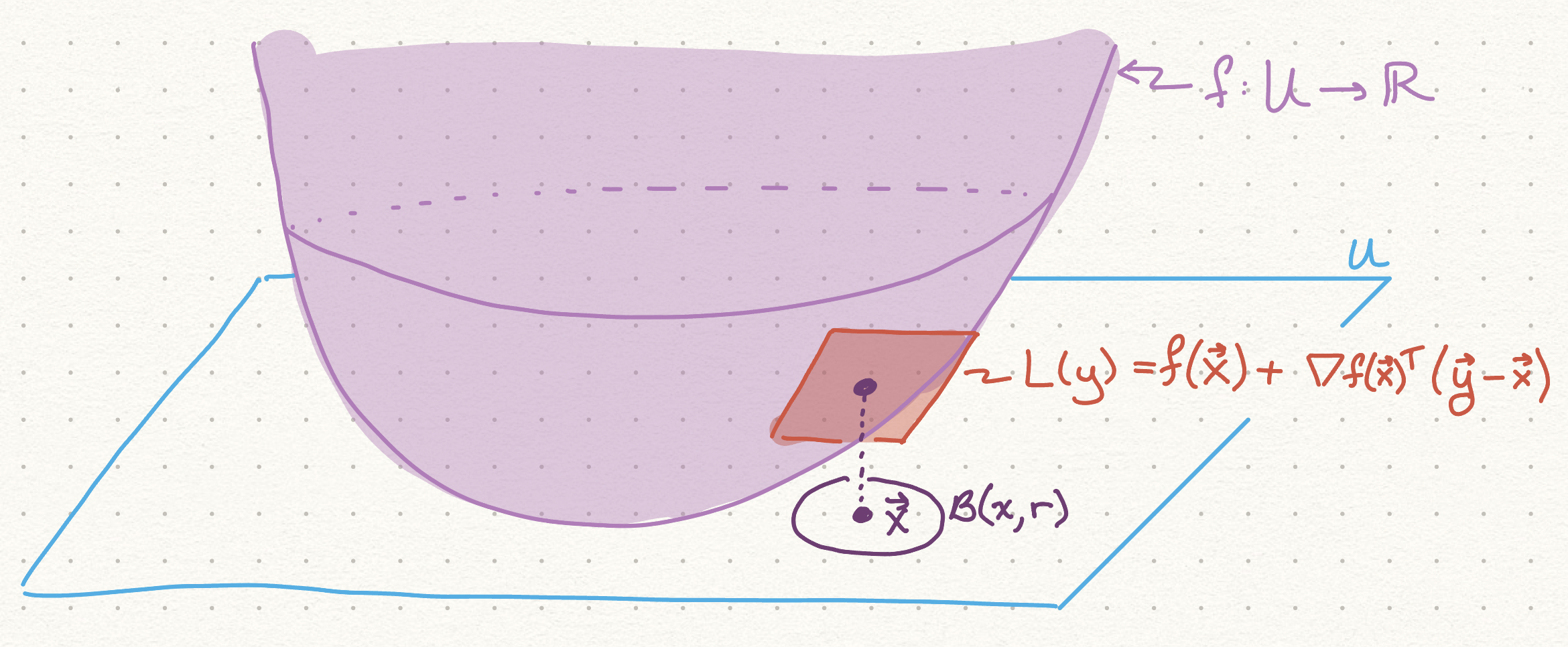
Linear Approximation Theorem#
Theorem (Linear Approximation Theorem):
Let \(f : U \to \mathbb{R}\) be a twice continuously differentiable function over an open set \(U \subseteq \mathbb{R}^n\).
Let \(\mathbf{x} \in U\), \(r > 0\) satisfy \(B(\mathbf{x}, r) \subseteq U\).
Then for any \(\mathbf{y} \in B(\mathbf{x}, r)\) there exists \(\boldsymbol{\xi} \in [\mathbf{x}, \mathbf{y}]\) such that
Quadratic Approximation Theorem#
Theorem (Quadratic Approximation Theorem):
Let \(f : U \to \mathbb{R}\) be a twice continuously differentiable function over an open set \(U \subseteq \mathbb{R}^n\).
Let \(\mathbf{x} \in U\), \(r > 0\) satisfy \(B(\mathbf{x}, r) \subseteq U\).
Then for any \(\mathbf{y} \in B(\mathbf{x}, r)\):