
Worksheet Chapter 3, Part 2#
✅ Put your name here.
✅ Put your group number here.
Topics#
This section focuses on Ch 3 from Beck
Regularized Least Squares
Tikhonov (Quadratic) Regularization
Denoising using regularized least squares
%matplotlib inline
import matplotlib.pylab as plt
import numpy as np
import scipy as sp
from scipy.sparse import diags
Regularized least squares#
Last time we solved problems of the form
Today’s change is that we are going to add a regularization term, so we are going to solve the regularized least squares (RLS) problem
\(\lambda\) is the regularization paramter. If it is 0, we are just doing ordinary least squares again. The larger \(\lambda\) is, the more weight is given to the regularization function.
\(R(\mathbf{x})\) is some chosen function of the input vector \(\mathbf{x}\).
We are generally going to work with quadratic regularization (also called Tikhonov regularization) where \(R(\mathbf{x}) = \|D\mathbf{x}\|^2\). If \(A^\top A + \lambda D^\top D \succ 0\), then the RLS solution is given by
❓❓❓ Question ❓❓❓: In a moment we will be using the regularization term
For this setting, what is \(\mathbf{D}\)? What does \(x_{RLS}\) simplify to in this case?
✎ Answer the question here.
Solution
\(x_{RLS} = (A^\top A + \lambda I)^{-1} A^\top b.\)
Example#
Let
and \(\mathbf{b}\) is a noisy measurement of \(\mathbf{A}\mathbf{x}_{true}\), that is,
where \(\mathbf{e}\) is randomly generated from a standard normal distributtion with zero mean and standard deviation of \(0.01\).
We don’t actually know \(\mathbf{e}\), so we are assuming someone handed us \(\mathbf{A}\) and \(\mathbf{b}\) and our goal is to find \(\mathbf{x}\) to minimize
A0 = np.array([[2, 3, 4], [3, 5, 7], [4, 7, 10]])
A = A0 + 1e-3 * np.eye(3)

print(f"A = \n{A}")
x_true = np.array([1, 2, 3]).T
b = A@x_true + 0.01 * np.random.randn(3)
print("\n")
print(f"b = {b}")
A =
[[ 2.001  3.     4.   ]
 [ 3.     5.001  7.   ]
 [ 4.     7.    10.001]]


b = [20.00090976 33.99555657 47.99461542]
❓❓❓ Question ❓❓❓:
Write code to find the least squares solution \(x_{LS}\) for
Print your answer. Is it close to true value of
x? If not, why do you think so?
# Enter your code below.
✎ Answer the question here.
Our found \(\mathbf{x}\) is nowhere close to \(\mathbf{x}_{true}\) even though \(\mathbf{A}\) is full rank. It is because the condition number of \(\mathbf{A}\) is very large. The condition number is the ratio of the largest to the smallest eigenvalues of \(\mathbf{A}\).
❓❓❓ Question ❓❓❓:
Write code below to find the eigenvalues of \(A\)
Compute the ratio of the largest to the smallest to check that this ratio, which is the condition number, is indeed large.
# Enter code below.
To control the output of the least squares solution, we instead optimize a regularized version, which minimizes
❓❓❓ Question ❓❓❓: Use what you figured out in the first section to solve for \(\mathbf{x}_{RLS}\) in the case \(\lambda = 0.1\) by multiplying the available matrices. Is your solution close to \(x_{true}\) now?
# Your code here
Denoising#
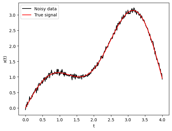
The denoising problem aims to remove noise or corruptions in a signal. Say you are given a time series \(\mathbf{b} \in \mathbf{R}^n\), and you think it came from a noisy sample of some real data \(\mathbf{x}_{true} \in \mathbf{R}^n\) plus some noise \(\mathbf{w} \in \mathbf{R}^n\). That is
Your job is to find a good guess for \(\mathbf{x}\) but you don’t have much to go on since you know nothing about \(\mathbf{w}\).
Let’s set up an example.
n = 300
t = np.linspace(0, 4, n)
x_true = np.sin(t) + t*(np.cos(t)**2)
b = x_true + 0.05 * np.random.randn(n)
plt.plot(t, b, 'k', label='Noisy data')
plt.plot(t, x_true, 'r-', label='True signal')
plt.xlabel('t')
plt.ylabel('x(t)')
plt.legend();
The least squares problem for \(\mathbf{x} \approx \mathbf{b}\), where we are solving \(A\mathbf{x} = \mathbf{b}\) for just \(A\) equal to the identity matrix, is
However, obviously the minimizer of the problem is \(\mathbf{x} = \mathbf{b}\), so there’s really no point in studying that at all. Instead, we can use the solution of the regularization version
to get more useful information.
Choosing the regularization term#
We know that we want the signal to be smooth, but what does that mean? For us, we’re going to try to find \(\mathbb{x}\) so that adjacent values \(x_i\) and \(x_{i+1}\) are close together, meaning \(|x_i-x_{i+1}|\) is small. This can be required by using a regularization term like this:
But that doesn’t look like our \(\|D\mathbf{x}\|^2\) term yet so we need to fix it.
In this case, we choose to use the “first order Tikhanov regularization matrix”
❓❓❓ Question ❓❓❓:
Write down by hand the matrix \(L\) for \(n=4\). Note you should have an \((n-1) \times n = 3 \times 4\) matrix.
Once you have written it down, uncomment the code below to check that you have the same matrix.
# Here's one way to get the matrix L

n = 4
L = diags([1,-1], offsets = [0,1], shape=(n-1,n)).toarray()

L
/var/folders/j9/kbv0jxbn7458fwg4nvr4rlkm0000gn/T/ipykernel_71639/1214235867.py:4: FutureWarning: Input has data type int64, but the output has been cast to float64.  In the future, the output data type will match the input. To avoid this warning, set the `dtype` parameter to `None` to have the output dtype match the input, or set it to the desired output data type.
  L = diags([1,-1], offsets = [0,1], shape=(n-1,n)).toarray()
array([[ 1., -1.,  0.,  0.],
       [ 0.,  1., -1.,  0.],
       [ 0.,  0.,  1., -1.]])
❓❓❓ Question ❓❓❓:
Now, again by hand, multiply \(\mathbf{L}\mathbf{x}\) for \(n=4\) where you can write
The result above should be a vector. What is \(\|L\mathbf{x}\|^2\)?
✎ Space for notes here.
Solution
The multiplication results in
Then the norm when no one tells you a subscript is just the 2-norm, so here it’s the square root of the sum of the entries squared. So, it’s
which is exactly what we wanted in the first place.
Back to the example#
Ok, so we were working with this data drawn below.
plt.plot(t, b, 'k', label='Noisy data')
plt.plot(t, x_true, 'r-', label='True signal')
plt.xlabel('t')
plt.ylabel('x(t)')
plt.legend();
❓❓❓ Question ❓❓❓: I’ve copied the code to make \(L\) below.
Add code to find the solution to the RLS problem when \(\lambda = 10\).
Plot your solution. What do you see?
### Complete the code below.

n = len(b)
L = diags([1,-1], offsets = [0,1], shape=(n-1,n)).toarray()

lam = 10

#Enter code below to find regularized least squares solution.


#Plot the solution
/var/folders/j9/kbv0jxbn7458fwg4nvr4rlkm0000gn/T/ipykernel_71639/614064222.py:4: FutureWarning: Input has data type int64, but the output has been cast to float64.  In the future, the output data type will match the input. To avoid this warning, set the `dtype` parameter to `None` to have the output dtype match the input, or set it to the desired output data type.
  L = diags([1,-1], offsets = [0,1], shape=(n-1,n)).toarray()
Effect of \(\lambda\)#
Next, we would like to study how the choice of the regularization parameter \(\lambda\) affects the solution.
❓❓❓ Question ❓❓❓: Write code below that solves for and plots the denoised signal for \(\lambda = [1, 10, 100, 1000]\) to compare with the true signal \(x_{true}\).
## Enter your code below.
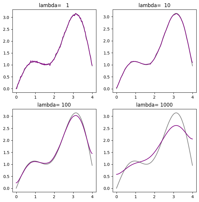
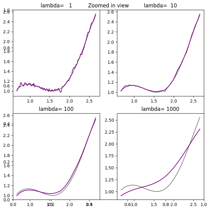
❓❓❓ Question ❓❓❓: What values of \(\lambda\) give you close enough solution to the clean signal? What happens when \(\lambda\) is too large?
✎ Answer the question here.
Solution
\(\lambda=10\) gives relatively clean solution. The result for \(\lambda = 1\) still looks noisy. For larger \(\lambda\) values, the solution starts deviating more from the clean signal.
Extra time#
If you have extra time, try this. Last class we did polynomial regression with ordinary least squares. For that data, add a quadratic regularization term. How does this change the learned function?
© Copyright 2025, The Department of Computational Mathematics, Science and Engineering at Michigan State University.