
Lecture 4-3: Gradient Method: Part 3#
Download the original slides: CMSE382-Lec4_3.pdf
Warning
This is an AI-generated transcript of the lecture slides and may contain errors or inaccuracies. Please refer to the original course materials for authoritative content.
Lipschitz Continuity#
Topics Covered#
Topics:
Review: Lipschitz continuity
Convergence of the gradient method
Lipschitz Continuity#
Definition: A continuously differentiable function \(f\colon \mathbb{R}^n \to \mathbb{R}\) is Lipschitz continuous if there exists an \(L > 0\) such that
for any \(\textbf{x}, \textbf{y} \in \mathbb{R}^n\).
If \(f\) is Lipschitz with constant \(L\), then it is Lipschitz with any constant \(L' \geq L\).
We are usually interested in the smallest Lipschitz constant.
Lipschitz Gradient#
We assume that \(f\colon \mathbb{R}^n \to \mathbb{R}\) is continuously differentiable and that \(\nabla f\) is Lipschitz continuous:
There exists an \(L > 0\) such that:
If \(\nabla f\) is Lipschitz with constant \(L\), then it is Lipschitz with any constant \(L' \geq L\).
The class of functions over a set \(D\) whose gradient satisfies the Lipschitz condition with constant \(L\) is denoted \(C^{1,1}_{L}(D)\).
\(C^{1,1}_{L}(D)\) is the class of functions “C-one-comma-one \(L\)-Lipschitz”.
If we don’t care about the value of \(L\), we write \(C^{1,1}(D)\) to denote functions that are Lipschitz for some \(L\).
Theorem: \(f \in C^{1,1}_L\) if and only if \(\|\nabla^2f(\textbf{x})\|\leq L\) for any \(\textbf{x} \in \mathbb{R}^n\).
Examples of \(C^{1,1}\) Functions#
Linear functions: Given \(\textbf{a} \in \mathbb{R}^n\), \(f(\textbf{x}) = \textbf{a}^\top\textbf{x}\) is in \(C^{1,1}\).
Quadratic functions: If \(\textbf{A}\) is an \(n\times n\) symmetric matrix, \(\textbf{b}\in \mathbb{R}^n\), and \(c\in \mathbb{R}\), then \(f(\textbf{x}) = \textbf{x}^\top\textbf{A}\textbf{x}+2\textbf{b}^\top+c\) is a \(C^{1,1}\) function (\(\|\nabla^2 f\| = 2 \|A\|\)).
Choice of norm:
The value of the Lipschitz constant \(L\) depends on the norm used
The choice of the norm does not impact Lipschitz continuity, only the value of \(L\).
Convergence of Gradient Method#
Convergence of the Gradient Method#
Given an unconstrained optimization problem
When will gradient descent converge?
How many iterations to reach the stopping criteria \(\|\nabla f(\textbf{x}_k)\|^2 < \varepsilon\)?
Convergence Theorem#
Theorem: Let \(f \in C^{1,1}_L(\mathbb{R}^n)\), and let \(\{\textbf{x}_k\}_{k\geq0}\) be the sequence generated by the gradient method for solving \(\min\limits_{\textbf{x}\in\mathbb{R}^n}f(\textbf{x})\) with one of the following stepsize strategies:
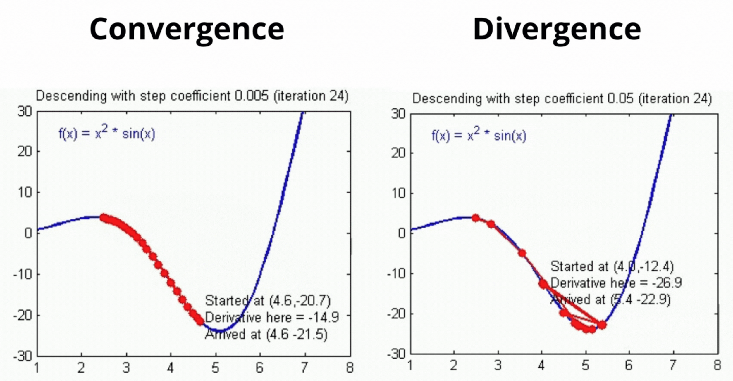
constant stepsize \(\bar{t} \in (0,\frac{2}{L})\)
exact line search
backtracking procedure with \(s \in \mathbb{R}_{++}, \alpha \in (0,1)\), and \(\beta \in (0,1)\).
Assume there exists \(m\in \mathbb{R}\) such that \(f(\textbf{x}) > m\) for all \(\textbf{x} \in \mathbb{R}^n\). Then:
(a) The sequence \(\{f(\textbf{x}_k)\}_{k \geq 0}\) is nonincreasing. In addition, for any \(k \geq 0\), \(f(\textbf{x}_{k+1}) < f(\textbf{x}_k)\) unless \(\nabla f(\textbf{x}_k) = \textbf{0}\).
(b) \(\nabla f(\textbf{x}_k) \to \textbf{0}\) as \(k \to \infty\).
Cannot guarantee convergence to a global optima, but can show convergence to a stationary point.
Rate of Convergence of Gradient Norms#
Theorem: Under the setting of the previous theorem, let \(f^\ast\) be the limit of the convergent sequence \(\{f(\textbf{x}_k)\}_{k \geq 0}\). Then for \(n+1\) iterations \(\exists k\) such that
where
Independent of the data vector size \(d\) (but \(L\) can grow with \(d\)).
Rate of Convergence and Advantages/Limitations#
How many iterations to reach the stopping criteria \(\|\nabla f(\textbf{x}_k)\|^2 < \varepsilon\)?
\(\|\nabla f(\textbf{x}_k)\|^2 \leq \frac{f(\textbf{x}_0)-f^\ast}{M(n+1)}\), so for \(\|\nabla f(\textbf{x}_k)\|^2 \leq \varepsilon\):
We need \((n+1)\) of order \(1/\varepsilon\) for \(\|\nabla f(\textbf{x}_k)\|^2 < \varepsilon\)
In practice, gradient descent converges much faster
Advantages and limitations of gradient descent method:
(+) Simple and easy to implement
(+) Very fast for well-conditioned objective functions (can find global optima for convex functions)
(-) Often slow for non-convex problems
(-) Inapplicable to non-differentiable functions