
Lecture 10-3: Optimality Conditions for Linearly Constrained Problems#
Download the original slides: CMSE382-Lec10_3.pdf
Warning
This is an AI-generated transcript of the lecture slides and may contain errors or inaccuracies. Please refer to the original course materials for authoritative content.
This Lecture#
Topics:
Orthogonal projection onto an affine space
Orthogonal projection onto hyperplanes
Announcements:
Quiz today!
Orthogonal projection using KKT conditions#
Recall: Orthogonal projection#
Definition (Recall: Orthogonal projection operator)
Given a nonempty closed convex set \(C\), the orthogonal projection operator \(P_C:\mathbb{R}^n \to C\) is defined by
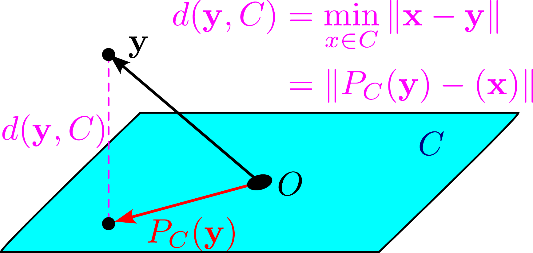
Returns the vector \(\mathbf{x}\) in \(C\) that is closest to input vector \(\mathbf{y}\).
Is a convex optimization problem:
Orthogonal Projection onto an Affine Space with KKT conditions#
Let \(C\) be an affine space
where \(A\in \mathbb{R}^{m\times n}\) and \(\mathbf{b} \in \mathbb{R}^m\). Assume that the rows of \(A\) are linearly independent.
Given \(\mathbf{y} \in \mathbb{R}^n\), find \(P_C(\mathbf{y})\) which is the solution to the optimization problem
The Langrangian simplifies to
for \(\boldsymbol{\mu} \in \mathbb{R}^m\)
The KKT stationarity conditions are:
Solving with \({A}\mathbf{x} = \mathbf{b}\) gives
Orthogonal Projection onto a hyperplane with KKT conditions#
Given a hyperplane
Given \(\mathbf{y} \in \mathbb{R}^n\), find \(P_H(\mathbf{y})\) which is the solution to the optimization problem
Special case of orthogonal projection onto an affine space with \(A=\mathbf{a}^{\top}\) and \(\mathbf{b}=b\).
Replacing in the previous solution gives