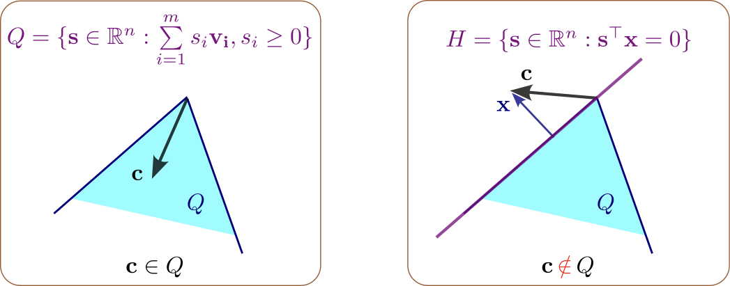
Lecture 10-1: Optimality Conditions for Linearly Constrained Problems

Lecture 10-1: Optimality Conditions for Linearly Constrained Problems#

Download the original slides: CMSE382-Lec10_1.pdf

Warning

This is an AI-generated transcript of the lecture slides and may contain errors or inaccuracies. Please refer to the original course materials for authoritative content.

This Lecture#

Topics:

Optimality conditions: motivation
Separation and alternative theorems
KKT conditions
Lagrangian function

Announcements:

Quiz Weds April 1

Optimality Conditions#

Optimality conditions#

Strict separation theorem#

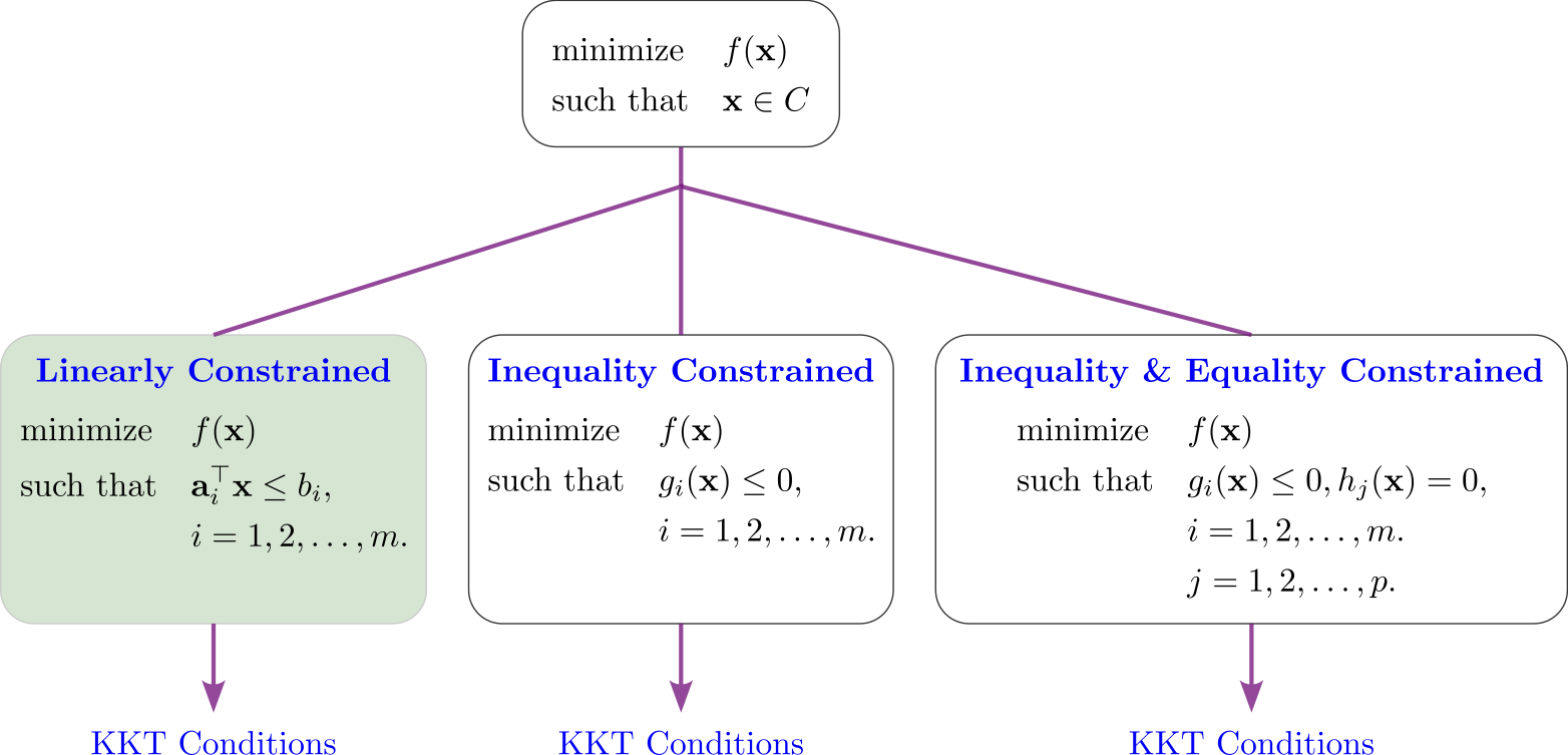
Theorem (Strict separation theorem)

Let \(C \subseteq \mathbb{R}^n\) be a nonempty closed and convex set, and let \(\mathbf{y} \notin C\). Then there exist \(\mathbf{p} \in \mathbb{R}^n\backslash \{\mathbf{0}\}\) and \(\alpha \in \mathbb{R}\) such that

\[ \mathbf{p}^{\top} \mathbf{y} > \alpha, \hspace{0.1in} \text{ and } \hspace{0.1in} \mathbf{p}^{\top} \mathbf{x} \le \alpha \text{ for all } \mathbf{x} \in C. \]

Meaning: Given \(C\) and \(\mathbf{y}\) as above, it is possible to draw a hyperplane separating \(\mathbf{y}\) and \(C\).

Farkas’ lemma#

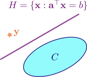
Lemma (Farkas’ lemma)

Let \(\mathbf{c} \in \mathbb{R}^n\) and \(A \in \mathbb{R}^{m\times n}\). Then exactly one of the following systems has a solution:

There is an \(\mathbf{x} \in \mathbb{R}^n\) such that \(A \mathbf{x} \le \mathbf{0}\), \(\mathbf{c}^{\top} \mathbf{x} > 0\).
There is a \(\mathbf{y} \in \mathbb{R}^m\) such that \(A^{\top} \mathbf{y} = \mathbf{c}\), \(\mathbf{y} \geq 0\).

Farkas’ lemma v2. Gordan’s alternative theorem#

Lemma (Farkas’ lemma—second formulation)

Let \(\mathbf{c} \in \mathbb{R}^n\) and \(A \in \mathbb{R}^{m\times n}\). Then the following two claims are equivalent.

The implication \(A \mathbf{x} \leq \mathbf{0}\) \(\Rightarrow\) \(\mathbf{c}^{\top} \mathbf{x} \leq 0\) holds true.
There exists \(\mathbf{y} \in \mathbb{R}^M_{+}\) such that \(A^T \mathbf{y} = \mathbf{C}\).

Theorem (Gordon’s alternative theorem)

Let \(A \in \mathbb{R}^{m\times n}\). Then exactly one of the following two systems has a solution:

\(A \mathbf{x} < 0\).
There exists \(\mathbf{p} \neq \mathbf{0}\) that satisfies \(A^{\top} \mathbf{p} = \mathbf{0}\), \(\mathbf{p} \geq \mathbf{0}\)

KKT for linearly constrained problems#

Theorem (Necessary optimality conditions)

Consider the minimization problem

\[\begin{split} \begin{aligned} (\text{P}) \quad &\min_{\mathbf{x}} f (\mathbf{x}) \\ &\text{s.t.} \quad \mathbf{a}_i^T \mathbf{x} \leq b_i, \quad i = 1, 2, \dots, m, \end{aligned} \end{split}\]

where \(f\) is continuously differentiable over \(\mathbb{R}^n\), \(a_1, a_2, \dots, a_m \in \mathbb{R}^n\), \(b_1, b_2, \dots, b_m \in \mathbb{R}\), and let \(\mathbf{x}^*\) be a local minimum point of (P). Then there exist \(\lambda_1, \lambda_2, \dots, \lambda_m \geq 0\) such that

\[ \nabla f (\mathbf{x}^*) + \sum_{i=1}^{m}\lambda_i a_i = 0, \quad \text{ and } \quad \lambda_i(\mathbf{a}_i^T \mathbf{x}^* - b_i) = 0, \quad i = 1, 2, \dots, m. \]

\(\lambda_1,\ldots,\lambda_m\) are Lagrange multipliers. Non-negative for minimization with inequality constraints.

KKT for convex linearly constrained problems#

Theorem (Necessary and sufficient optimality conditions)

Consider the minimization problem

\[\begin{split} \begin{aligned} (\text{P}) \quad &\min_{\mathbf{x}} f (\mathbf{x}) \\ &\text{s.t.} \quad \mathbf{a}_i^T \mathbf{x} \leq b_i, \quad i = 1, 2, \dots, m, \end{aligned} \end{split}\]

where \(f\) is a convex continuously differentiable over \(\mathbb{R}^n\), \(a_1, a_2, \dots, a_m \in \mathbb{R}^n\), \(b_1, b_2, \dots, b_m \in \mathbb{R}\), and let \(\mathbf{x}^*\) be a feasible solution of (P). Then \(\mathbf{x}^*\) is an optimal solution of (P) if and only if there exist \(\lambda_1, \lambda_2, \dots, \lambda_m \geq 0\) such that

\[ \nabla f (\mathbf{x}^*) + \sum_{i=1}^{m}\lambda_i a_i = 0, \quad \text{ and } \quad \lambda_i(\mathbf{a}_i^T \mathbf{x}^* - b_i) = 0, \quad i = 1, 2, \dots, m. \]

The condition \(\lambda_i(\mathbf{a}_i^T \mathbf{x}^* - b_i) = 0, \quad i = 1, 2, \dots, m\) is called the complementary slackness condition.

The Lagrangian function#

Definition (The Lagrangian function)

Consider the Nonlinear Programming Problem (NLP)

\[ (\text{NLP}) \quad \min_{\mathbf{x}} f (\mathbf{x}) \quad \text{s.t.} \quad \{g_i(\mathbf{x}) \leq 0\}_{i=1}^m, \quad \{h_j(\mathbf{x}) = 0\}_{j=1}^p, \]

where \(f\), and all the \(g_i\) and \(h_j\) are continuously differentiable over \(\mathbb{R}^n\).

The associated Lagrangian function is of the form

\[\begin{split} \begin{aligned} L(&\mathbf{x},\boldsymbol{\lambda},\boldsymbol{\mu}) = \\ & f(\mathbf{x}) + \sum\limits_{i=1}^m{\lambda_i g_i(\mathbf{x})} + \sum\limits_{j=1}^p{\mu_j h_j(\mathbf{x})}. \end{aligned} \end{split}\]

The necessary KKT condition (stationarity condition) is

\[\begin{split} \begin{aligned} \nabla_{\mathbf{x}}&L(\mathbf{x},\boldsymbol{\lambda},\boldsymbol{\mu}) = \\ &\nabla f(\mathbf{x}) + \sum\limits_{i=1}^m{\lambda_i \nabla g_i(\mathbf{x})} + \sum\limits_{j=1}^p{\mu_j \nabla h_j(\mathbf{x})}=\mathbf{0}. \end{aligned} \end{split}\]

The Lagrangian function for linearly constrained optimization#

Recall the minimization problem with linear constraints

\[ (\text{Q}) \quad \min_{\mathbf{x}} f (\mathbf{x}) \quad \text{s.t.} \quad A \mathbf{x} \leq \mathbf{b}, \quad C \mathbf{x} = \mathbf{d}. \]

The associated Lagrangian function is of the form

\[ L(\mathbf{x},\boldsymbol{\lambda},\boldsymbol{\mu}) = f(\mathbf{x}) + \boldsymbol{\lambda}^{\top}(A \mathbf{x}-\mathbf{b}) + \boldsymbol{\mu}^{\top}(C \mathbf{x}-\mathbf{d}). \]

The necessary KKT condition \(\nabla f(\mathbf{x}^*) + \sum_{i=1}^{m} \lambda_i \mathbf{a}_i + \sum_{j=1}^{p} \mu_j \mathbf{c}_j = \mathbf{0}\) can be written in terms of the Lagrangian as

\[ \nabla_{\mathbf{x}} L(\mathbf{x},\boldsymbol{\lambda}, \boldsymbol{\mu}) = \nabla f(\mathbf{x}) + A^{\top} \boldsymbol{\lambda} + C^T \boldsymbol{\mu}=\mathbf{0}. \]

Steps for finding the stationary points for a linearly constrained problem#

Write the problem in the standard form

\[ \min_{\mathbf{x}} f (\mathbf{x}) \quad \text{s.t.} \quad A \mathbf{x} \leq \mathbf{b}, \quad C \mathbf{x} = \mathbf{d}. \]

Write down the Lagrangian function