
Lecture 5-2: Newton’s Method: Part 2#
Download the original slides: CMSE382-Lec5_2.pdf
Warning
This is an AI-generated transcript of the lecture slides and may contain errors or inaccuracies. Please refer to the original course materials for authoritative content.
Damped Newton’s Method#
Topics Covered#
Topics:
Damped Newton’s method
Cholesky factorization
Hybrid gradient-Newton method
Announcements:
Homework 2 posted, due Thursday, Feb 12 at 11:59pm
Midterm 1 on Wednesday, Feb 18.
No office hours Friday, Feb 13.
Damped Newton Method - Motivating Example#
Consider the function \(f(x,y) = \sqrt{x^2+1}+\sqrt{y^2+1}\) whose optimal solution is \((0,0)\).
There is NO \(m > 0\) such that \(\lambda_{\min}(\nabla^2 f(\textbf{x})) \geq m\) for any \(\mathbf{x} \in \mathbb{R}^n\)
Slow convergence:
Divergence:
Descent of the generated sequence is not guaranteed even when \(\nabla^2 f(\mathbf{x}) > 0\).
Rectify by introducing a step size \(t_k\) (Damped Newton’s method).
Damped Newton’s Method Algorithm#
Input: \(\varepsilon > 0\) tolerance parameter
Initialization: Pick \(\textbf{x}_0 \in \mathbb{R}^n\) arbitrarily
General step: For any \(k = 0, 1, 2, \ldots\), do:
Compute the Newton direction \(\textbf{d}_k\), which is the solution to the linear system \(\nabla^2 f(\textbf{x}_k)\textbf{d}_k = -\nabla f(\textbf{x}_k)\)
Pick \(t_k\) using constant stepsize, exact line search, or backtracking
Set \(\textbf{x}_{k+1} = \textbf{x}_k+t_k\textbf{d}_k\)
If \(\|\nabla f(\textbf{x}_{k+1})\| < \varepsilon\), stop and output \(\textbf{x}_{k+1}\).
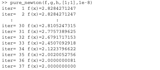
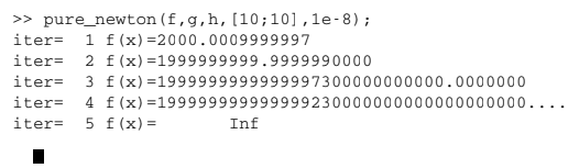
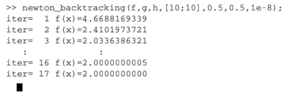
Damped Newton Method - Revisiting the Example#
Revisiting the previous example: \(f(x,y) = \sqrt{x^2+1}+\sqrt{y^2+1}\)
There is NO \(m > 0\) such that \(\lambda_{\min}(\nabla^2 f(\textbf{x})) \geq m\) for any \(\mathbf{x} \in \mathbb{R}^n\)
Pure Newton’s Divergence:
Damped Newton’s Convergence:
Cholesky Decomposition#
Cholesky Decomposition#
When \(A\) is symmetric and positive definite, it has a Cholesky decomposition given by
where \(L\) is a lower triangular matrix (a matrix with zeros everywhere above the diagonal).
If \(A\) is diagonal, the Cholesky decomposition represents the matrix square root:
Example: \(A=\begin{bmatrix}9 & 0\\ 0 & 25\end{bmatrix}\), \(L = A^{\frac{1}{2}}=\begin{bmatrix} 3 & 0\\ 0 & 5\end{bmatrix}\)
Verify: \(L L^T=\begin{bmatrix} 3 & 0\\ 0 & 5\end{bmatrix} \cdot \begin{bmatrix} 3 & 0\\ 0 & 5\end{bmatrix} = \begin{bmatrix}9 & 0\\ 0 & 25\end{bmatrix}\)
Hybrid Gradient-Newton Method#
Hybrid Gradient-Newton Method - Motivation#
Motivation:
Newton’s method assumes that \(\nabla^2 f(\mathbf{x})>0\).
Gradient Descent does not use the Hessian.
We avoid the assumption \(\nabla^2 f(\mathbf{x})>0\) by constructing a hybrid method.
The hybrid gradient-Newton method:
Does not require the Hessian to be positive definite
Is likely to converge faster than the gradient method
Approach: At each iteration, determine if \(\nabla^2f(\textbf{x}_k) \succ 0\)
If \(\nabla^2f(\textbf{x}_k) \succ 0\), use a Newton step
Otherwise, use a gradient descent step
Hybrid Gradient-Newton Method Algorithm#
Input: \(\varepsilon>0\) tolerance parameter, method for finding stepsize \(t\) (constant step size, exact line search, or backtracking)
Initialization: Pick \(\textbf{x}_0 \in \mathbb{R}^n\) arbitrarily
General step: For any \(k = 0,1,2, \ldots\), do:
If \(\nabla^2f(\textbf{x}_k) \succ 0\), then take \(\mathbf{d}_k\) as the solution to the system \(\nabla^2 f(\textbf{x}_k)\textbf{d}_k = -\nabla f(\textbf{x}_k)\). Else, set \(\textbf{d}_k = -\nabla f(\textbf{x}_k)\).
Pick stepsize \(t\) according to the input method
Set \(\textbf{x}_{k+1} = \textbf{x}_k+t_k\textbf{d}_k\)
If \(\|\nabla f(\textbf{x}_{k+1})\| \leq \varepsilon\), then stop and \(\textbf{x}_{k+1}\) is the output.