
Lecture 3-2: Least Squares: Part 2#
Download the original slides: CMSE382-Lec3_2.pdf
Warning
This is an AI-generated transcript of the lecture slides and may contain errors or inaccuracies. Please refer to the original course materials for authoritative content.
Regularized Least Squares#
Topics Covered#
Regularized least squares
Tikhonov regularization
De-noising
Ordinary Least Squares Approximation#
Definition: The residual sum of squares error (or total sum of square errors) is
The minimizer of this equation is the least squares estimate
Regularized Least Squares#
Definition: We add a regularization function \(R(\cdot)\) to OLS to obtain the regularized least squares function:
\(\lambda > 0\) determines the weight given to the regularization function.
\(R\) is chosen based on prior knowledge or desired behavior
When \(R(\mathbf{x})=0\), we recover ordinary least squares.
When \(R(\mathbf{x})=\|\mathbf{x}\|_2^2 = \sum_{i=1}^n x_i^2\), we have ridge regression.
When \(R(\mathbf{x})=\|\mathbf{x}\|_1\), we have LASSO regression.
Why Add Regularization?#
Why add \(R\)?
Can solve ill-posed problems.
Underdetermined systems have infinite solutions and OLS fails. Regularized least squares allows constraining the problem.
OLS focuses on reducing the error sum of squares, but can lead to poor fits in-between data points.
A regularization term can penalize big errors in-between data points for a better fit.
Regularization allows including prior knowledge into the model:
E.g., allows smoother fits for noisy data (denoising)
Tikhonov (Quadratic) Regularization#
Definition: When \(R(\mathbf{x})=\|D \mathbf{x} \|^2\), we have Tikhonov regularization. \(D\) is called the Tikhonov matrix.
We require that the null space of \(D\) must intersect the null space of \(A\) at \(\mathbf{0}\) for a unique solution.
Often \(D\) is a scalar multiple of the identity matrix.
Solving Tikhonov Regularization#
If \(\nabla^2 f = 2 (A^\top A+\lambda D^\top D) \succ 0\), then \(x_{\text{LS}}=(A^\top A + \lambda D^\top D)^{-1}A^\top \mathbf{b}\)
Tikhonov Regularization Choices#
Order |
\(R(\mathbf{x})\) |
Promotes |
|---|---|---|
zeroth |
\(|L_0 \, \mathbf{x}|^2\) |
small \(|\mathbf{x}|\), \(L_0\) is the identity matrix |
First |
\(|L_1\, \mathbf{x}|^2\) |
smoothness by minimizing 1st derivative |
Second |
\(|L_2 \, \mathbf{x}|^2\) |
smoothness by minimizing 2nd derivative |
First-order finite difference approximation:
Second-order finite difference approximation:
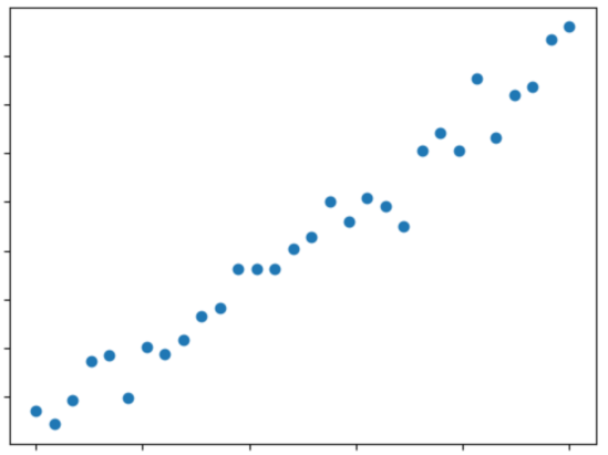
Noise#
Noisy data can be written as
where \(\textbf{x}\) is the signal vector and \(\mathbf{w}\) is the noise vector.
Problem Statement: Given \(\textbf{b}\), find a good estimate for \(\textbf{x}\)
Denoising Using Regularized Least Squares#
Idea: Directly incorporate prior knowledge that the solution is smooth.
Small difference between any two subsequent function values
Popular choice: \(R(\mathbf{x})=\sum\limits_{i=1}^{n-1}(x_i-x_{i+1})^2\)
Can write as a Tikhonov matrix: \(R(\mathbf{x})=\sum\limits_{i=1}^{n-1}(x_i-x_{i+1})^2=\|L\, \mathbf{x}\|^2\)
The regularized least squares problem becomes \(\min\limits_{\textbf{x}} \|\textbf{x}-\textbf{b}\|^2 + \lambda \|\mathbf{L}\textbf{x}\|^2\), with solution \(\textbf{x}_{\text{RLS}}(\lambda) = (\mathbf{I}+\lambda \mathbf{L}^\top \mathbf{L})^{-1}\textbf{b}\)