Lecture 12-1: Duality#

Download the original slides: CMSE382-Lec12_1.pdf

Warning

This is an AI-generated transcript of the lecture slides and may contain errors or inaccuracies. Please refer to the original course materials for authoritative content.


This Lecture#

Topics:

  • Motivation for Duality

  • Definition and weak duality

Announcements:

  • Homework 5 is due today, Friday April 10, at 11:59pm.


Motivation#

Duality Motivation#

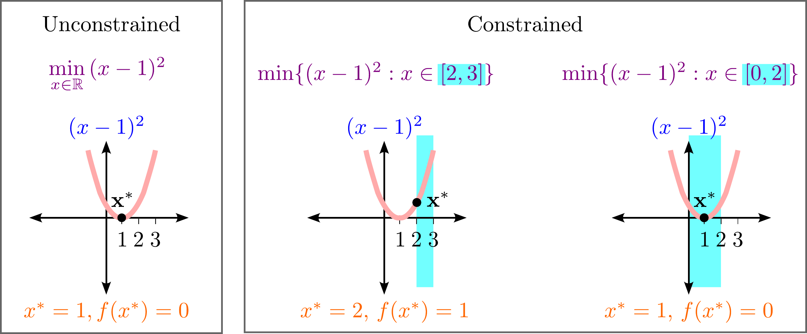
  • The optimal value (val) of unconstrained problem is lower bound for the constrained one.

    • \(\text{val}(unconstrained) \leq \text{val}(constrained)\)

  • Interested in finding lower bounds for constrained optimization by solving unconstrained problems.


Obtaining lower bounds#

Approach#1: Drop constraints

\[\begin{split} \begin{aligned} & \text{min} & & f(\mathbf{x}) = x^2+y^2+2x \\ & \text{such that} & & x+y=0. \end{aligned} \end{split}\]
\[ \begin{aligned} & \text{min} & & f(\mathbf{x}) = x^2+y^2+2x \end{aligned} \]
  • \(\text{val}(unconstrained) \leq \text{val}(constrained)\)

  • May not be the best lower bound.

  • We want the largest lower bound.

Desmos example


Obtaining lower bounds#

Approach#2: Optimize for best lower bounds

\[\begin{split} \begin{aligned} \llap{(P)} \hspace{0.1in} & \text{min} & & f(\mathbf{x}) + \mu h(\mathbf{x}) \\ &&&= x^2+y^2+2x+\mu(x+y)\\ & \text{s.t.} & & h(\mathbf{x})=x+y=0. \end{aligned} \end{split}\]
\[\begin{split} \begin{aligned} \llap{(P_\mu)} \hspace{0.1in} & \text{min} & & f(\mathbf{x}) + \mu h(\mathbf{x})\\ &&&= x^2+y^2+2x+\mu(x+y)\\ \end{aligned} \end{split}\]
  • \(\text{val}(\text{P}_{\mu}) \leq \text{val}(\text{P})\) for all \(\mu \in \mathbb{R}\).

  • Best lower bound is the solution to

\[\llap{($\text{D}$)} \hspace{0.2in} \max_{\mu}{\{\text{val}(P_{\mu})\}}.\]

Desmos example


Primal and Dual Problems#

Primal Problem

\[\begin{split} \begin{aligned} \llap{(P)} \hspace{0.2in} & \text{min} & & f(\mathbf{x}) \\ & \text{such that} & & h(\mathbf{x})=0. \end{aligned} \end{split}\]

Dual Problem

\[ \begin{aligned} \llap{(D)} \hspace{0.2in} & \text{max} & & \text{val}(P_{\mu}) \end{aligned} \]

Duality Definition#

Dual objective function#

Consider the general model referred to as the primal model

\[\begin{split} \begin{aligned} & f^* = \text{min} & & f(\mathbf{x}) \\ & \text{such that} & & g_i(\mathbf{x}) \leq 0, i=1,2,\ldots m, \\ & & & h_j(\mathbf{x}) = 0, j=1,2,\ldots p, \\ & & & \mathbf{x} \in X, \text{ where } X \subseteq \mathbb{R}^n, \end{aligned} \end{split}\]

and \(f, g_i,h_j\) are functions defined on \(X\).

The Lagrangian of the problem is

\[L(\mathbf{x},\boldsymbol{\lambda},\boldsymbol{\mu}) = f(\mathbf{x}) + \sum\limits_{i=1}^m{\lambda_i g_i(\mathbf{x})} + \sum\limits_{j=1}^p{\mu_j h_j(\mathbf{x})},\]

The dual objective function \(q: \mathbb{R}_+^m \times \mathbb{R}^p \to \mathbb{R} \cup \{-\infty\}\) is

\[q(\boldsymbol{\lambda},\boldsymbol{\mu})=\min_{x\in X}{L(\mathbf{x},\boldsymbol{\lambda},\boldsymbol{\mu})},\]

Dual problem#

Definition (Dual Problem)

The dual problem is given by

\[\begin{split} \begin{aligned} & q^* = \max\limits_{\boldsymbol{\lambda},\boldsymbol{\mu}} & & q(\boldsymbol{\lambda},\boldsymbol{\mu}) \\ & \text{such that} & & (\boldsymbol{\lambda},\boldsymbol{\mu}) \in \text{dom}(q), \end{aligned} \end{split}\]

where the domain of the dual objective function is

\[\text{dom}(q)=\{(\boldsymbol{\lambda},\boldsymbol{\mu}) \in \mathbb{R}_{+}^m \times \mathbb{R}^p: q(\boldsymbol{\lambda},\boldsymbol{\mu}) > -\infty\}.\]

Convexity of the dual problem#

Theorem (Convexity of the dual problem)

Let the dual problem be given by

\[\begin{split} \begin{aligned} & q^* = \max\limits_{\boldsymbol{\lambda},\boldsymbol{\mu}} & & q(\boldsymbol{\lambda},\boldsymbol{\mu}) \\ & \text{such that} & & (\boldsymbol{\lambda},\boldsymbol{\mu}) \in \text{dom}(q), \end{aligned} \end{split}\]

where \(f,g_1, \ldots, g_m, h_1,\ldots, h_p\) are functions defined on \(X \subseteq \mathbb{R}^n\), and \(q(\boldsymbol{\lambda},\boldsymbol{\mu})=\min_{\mathbf{x}\in X}{L(\mathbf{x},\boldsymbol{\lambda},\boldsymbol{\mu})}\). Then

(a) \(\text{dom}(q)\) is a convex set.

(b) \(q\) is a concave function over \(\text{dom}(q)\).

Maximizing a concave function over a convex set defines a convex problem.


Weak duality theorem#

Primal Problem

\[\begin{split} \begin{aligned} & f^* = \text{min} & & f(\mathbf{x}) \\ & \text{such that} & & g_i(\mathbf{x}) \leq 0, i=1,2,\ldots m, \\ & & & h_j(\mathbf{x}) = 0, j=1,2,\ldots p, \\ & & & \mathbf{x} \in X, \text{ where } X \subseteq \mathbb{R}^n, \end{aligned} \end{split}\]

and \(f, g_i,h_j\) are functions defined on \(X\).

Dual Problem

\[\begin{split} \begin{aligned} & q^* = \text{max} & & q(\boldsymbol{\lambda},\boldsymbol{\mu}) \\ & \text{such that} & & (\boldsymbol{\lambda},\boldsymbol{\mu}) \in \text{dom}(q), \end{aligned} \end{split}\]

where \(\text{dom}(q)=\{(\boldsymbol{\lambda},\boldsymbol{\mu}) \in \mathbb{R}_{+}^m \times \mathbb{R}^p: q(\boldsymbol{\lambda},\boldsymbol{\mu}) > -\infty\}\), and \(q(\boldsymbol{\lambda},\boldsymbol{\mu})=\min_{\mathbf{x}\in X}{L(\mathbf{x},\boldsymbol{\lambda},\boldsymbol{\mu})}\).

Theorem (Weak duality theorem)

Consider the primal problem and its dual. Then \(q^* \leq f^*\), where \(q^*, f^*\) are the optimal dual and primal values, respectively.