Lecture 6-3: Convex Sets: Part 3#
Download the original slides: CMSE382-Lec6_3.pdf
Warning
This is an AI-generated transcript of the lecture slides and may contain errors or inaccuracies. Please refer to the original course materials for authoritative content.
Feasible Region#
Topics Covered#
Topics:
Convex polytope
Feasible region
Basic feasible solutions
Extreme points
Review: Last Time#
Definition: A set \(C \subseteq \mathbb{R}^n\) is convex if for any \(\textbf{x}, \textbf{y} \in C\), the line segment \([\textbf{x}, \textbf{y}]\) is also in \(C\).
Definition: A set \(C \subseteq \mathbb{R}^n\) is a cone if for any \(\textbf{x} \in C\) and \(\lambda \geq 0\), we have \(\lambda \textbf{x} \in C\).
Theorem: A set \(C\) is a convex cone if and only if for any \(\textbf{x}, \textbf{y} \in C\) we have \(\textbf{x} + \textbf{y} \in C\).
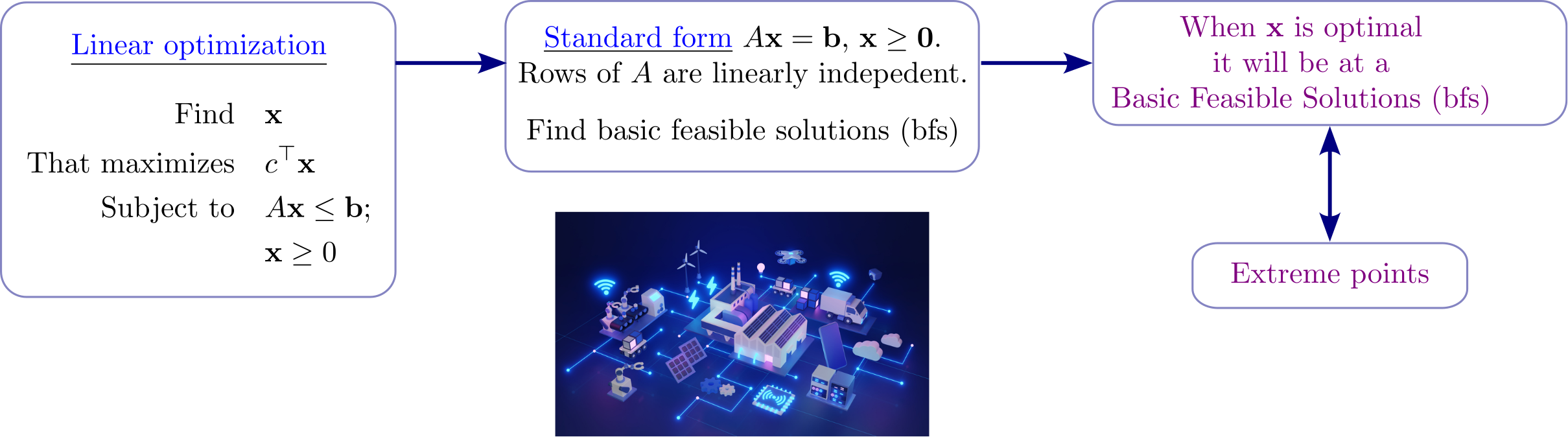
Motivation: Linear Optimization (Linear Programming)#
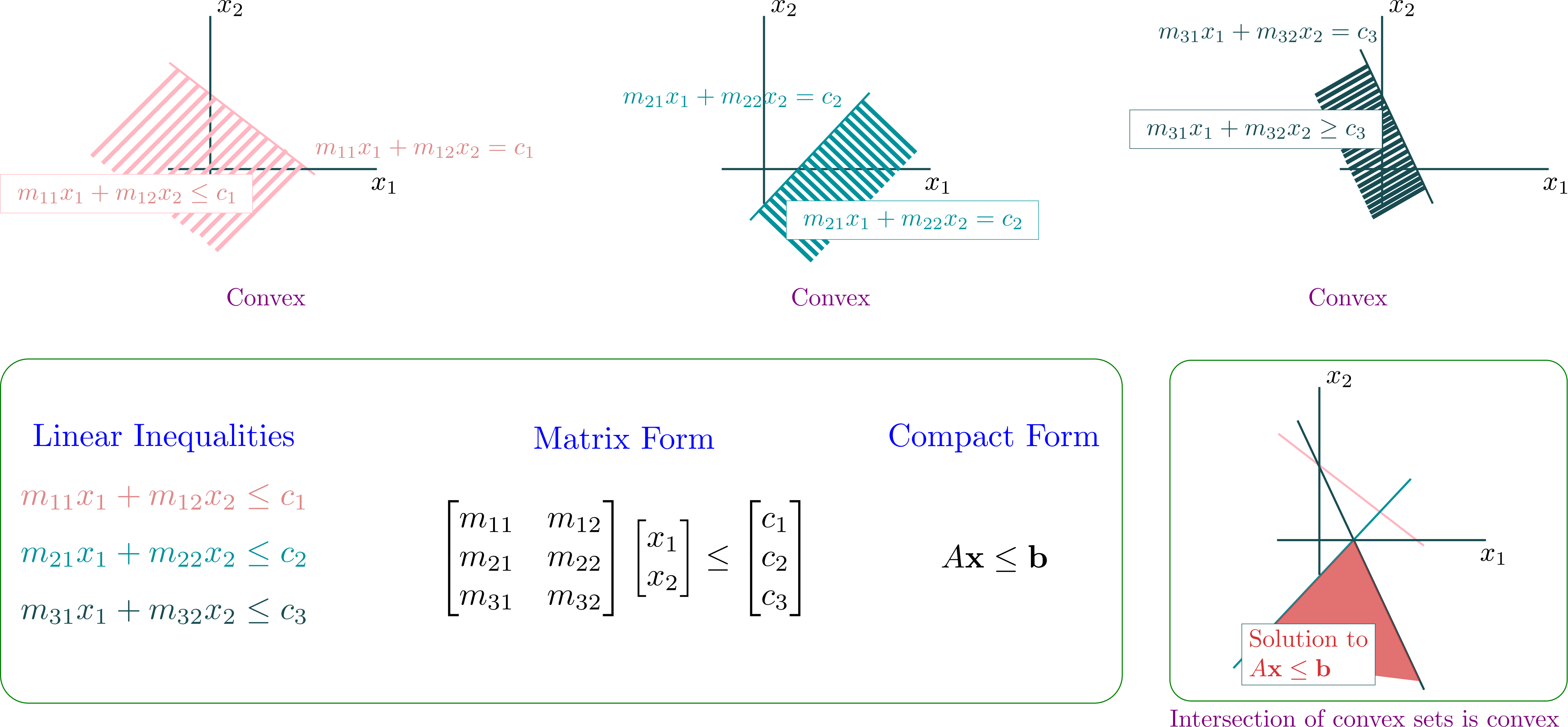
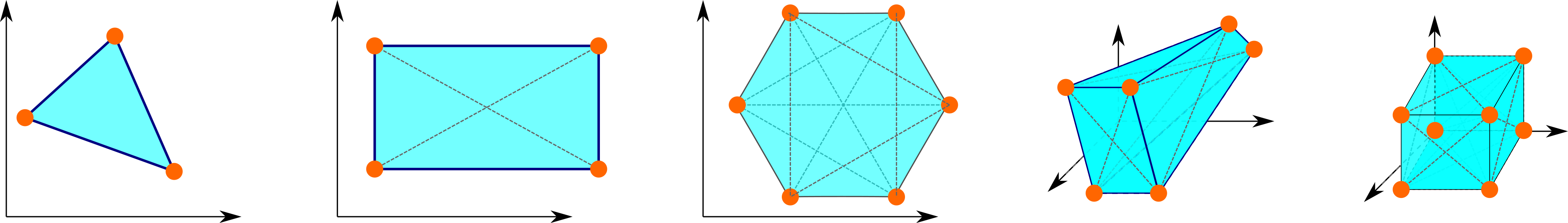
Polytopes#
Definition: A Polytope is a geometric object with flat faces.
It generalizes polyhedra to higher dimensions.
Polyhedron is a \(3\)-polytope.
Polygon is a \(2\)-polytope.
Definition: A polyhedron is a three-dimensional figure with flat polygonal faces, straight edges and sharp corners or vertices.

Convex Polytopes#
Definition: We define a convex polytope as the set
Feasible Region#
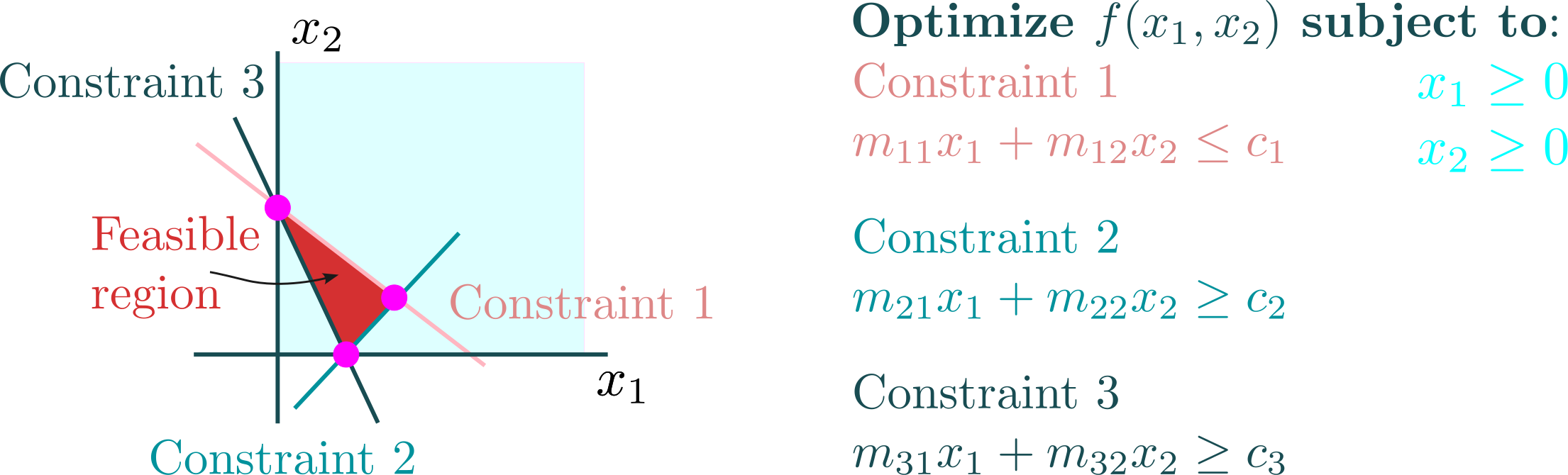
Definition: The feasible region of an optimization problem is the set of all possible points that satisfy the problem’s constraints.
It represents all the possible candidates for the optimization solution.
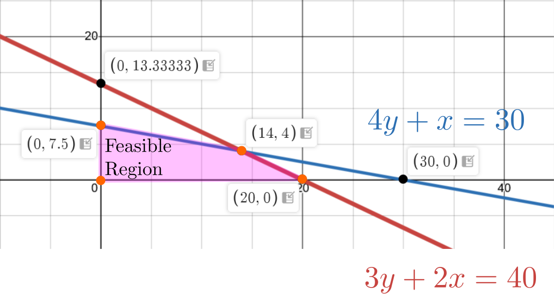
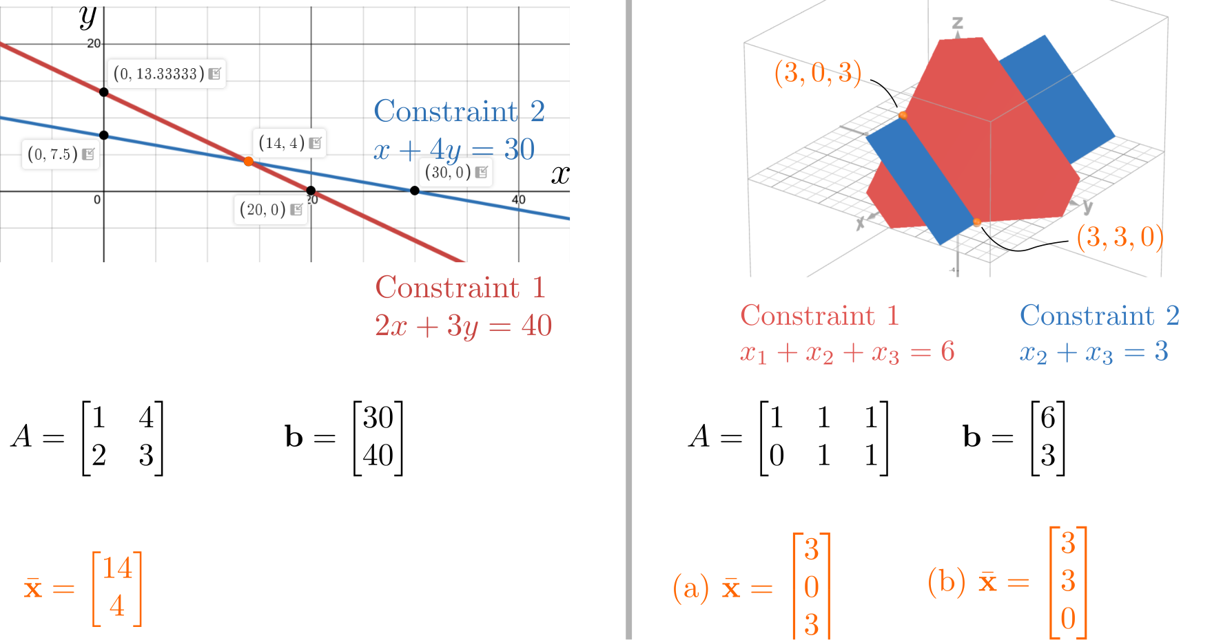
Example Feasible Region - 2D#
What is the feasible region for the linear system
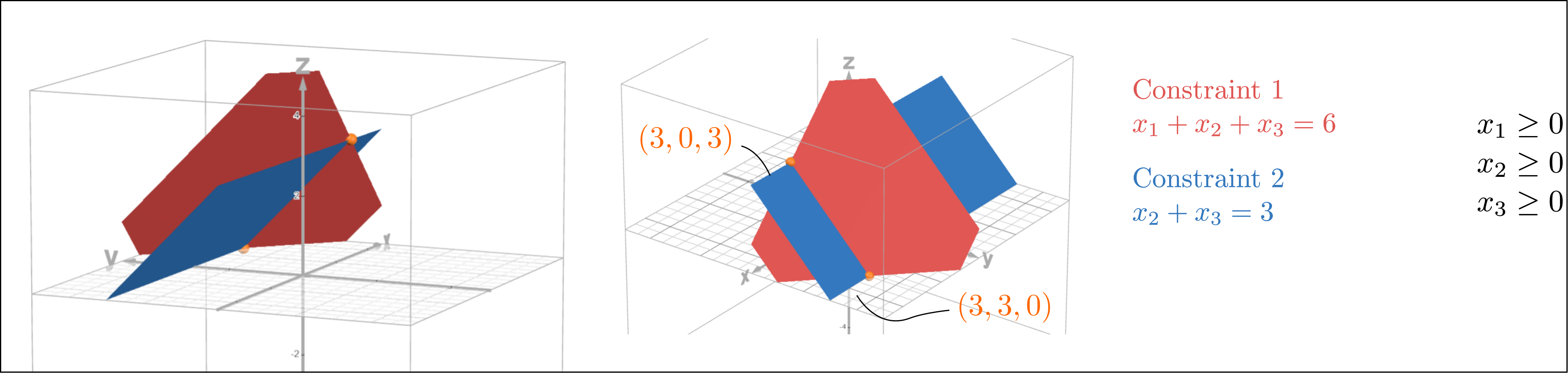
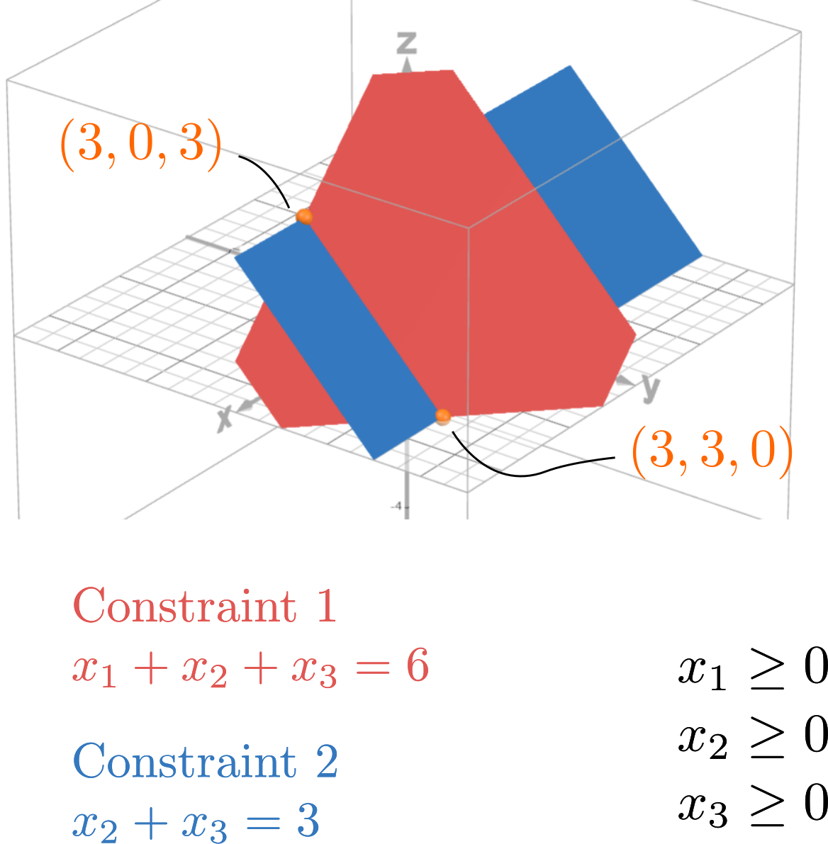
Example Feasible Region - 3D#
What is the feasible region for the linear system
Basic Feasible Solutions#
Basic Feasible Solutions#
Definition: Let
where \(A \in \mathbb{R}^{m\times n}\), \(b \in \mathbb{R}^m\), and \(A\)’s rows are linearly independent.
\(\overline{\textbf{x}}\) is a basic feasible solution (bfs) of \(P\) if the columns of \(\textbf{A}\) corresponding to the indices of the positive values of \(\overline{\textbf{x}}\) are linearly independent.
If \(P\) is non-empty, then it contains at least one bfs.
This is shown by using the conic representation theorem from last class.
A bfs has at most \(m\) non-zero elements.
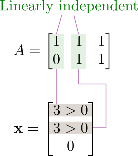
Example: Basic Feasible Solution#
Is \((x_1, x_2, x_3) = (3,3,0)\) a solution? Yes because \(3 + 3 + 0 = 6\); \(3 + 0 = 3\); \(3,3,0 \geq 0\).
Is it a bfs? Yes because the columns of \(A\) corresponding to the indices of the positive values of \(\overline{\textbf{x}}\) (which are \(x_1\) and \(x_2\)) are linearly independent.
Extreme Points#
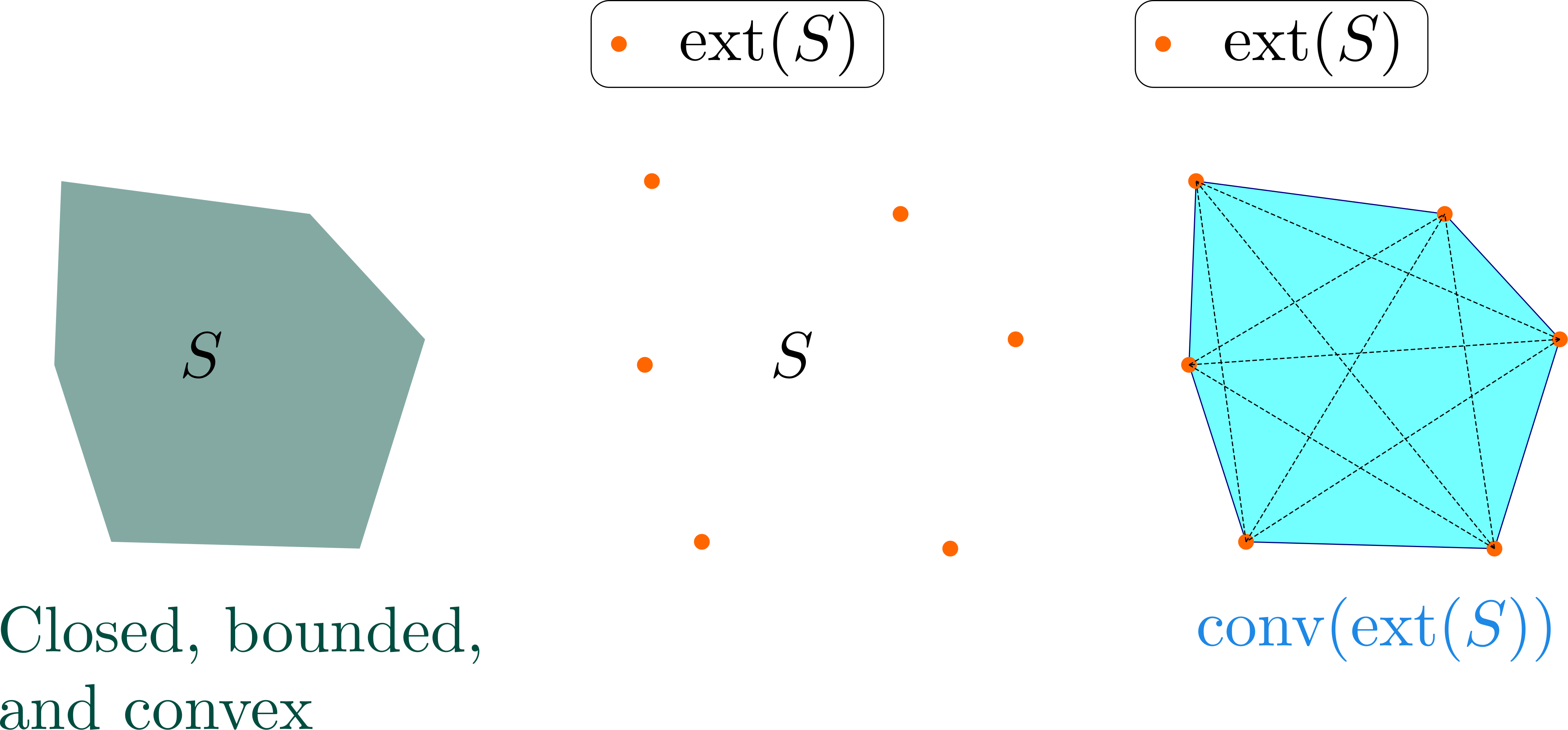
Definition: Let \(S\) be a convex set. A point \(\textbf{x} \in S\) is an extreme point of \(S\) if there do not exist two distinct points \(\textbf{x}_1, \textbf{x}_2 \in S\) and \(\lambda \in (0,1)\) such that \(\textbf{x} = \lambda\textbf{x}_1+(1-\lambda)\textbf{x}_2\).
It is a point in \(S\) that cannot be represented as a nontrivial convex combination of two different points in \(S\).
The set of all extreme points is denoted \(\text{ext}(S)\).
Equivalence of Extreme Points and BFS#
Theorem: Let \(P = \{\textbf{x} \in \mathbb{R}^n \mid \textbf{A}\textbf{x} = \textbf{b}, \textbf{x}\boldsymbol{\geq}\textbf{0}\}\), where \(\textbf{A} \in \mathbb{R}^{m \times n}\) has linearly independent rows and \(\textbf{b} \in \mathbb{R}^m\). Then \(\overline{\textbf{x}}\) is a basic feasible solution of \(P\) if and only if it is an extreme point of \(P\).
Extreme Points and Convex Hull#
Theorem: Let \(S \subseteq \mathbb{R}^n\) be a closed and bounded convex set. Then
A compact convex set is the convex hull of its extreme points.