Lecture 10-2: Optimality Conditions for Linearly Constrained Problems#
Download the original slides: CMSE382-Lec10_2.pdf
Warning
This is an AI-generated transcript of the lecture slides and may contain errors or inaccuracies. Please refer to the original course materials for authoritative content.
This Lecture#
Topics (Review):
KKT conditions
Lagrangian function
Added topic:
Active Constraints
Announcements:
Quiz Weds April 1
Optimality Conditions#
Optimality conditions#
KKT for linearly constrained problems#
Theorem (Necessary optimality conditions)
Consider the minimization problem
where \(f\) is continuously differentiable over \(\mathbb{R}^n\), \(a_1, a_2, \dots, a_m \in \mathbb{R}^n\), \(b_1, b_2, \dots, b_m \in \mathbb{R}\), and let \(\mathbf{x}^*\) be a local minimum point of (P). Then there exist \(\lambda_1, \lambda_2, \dots, \lambda_m \geq 0\) such that
\(\lambda_1,\ldots,\lambda_m\) are Lagrange multipliers. Non-negative for minimization with inequality constraints.
KKT for convex linearly constrained problems#
Theorem (Necessary and sufficient optimality conditions)
Consider the minimization problem
where \(f\) is a convex continuously differentiable over \(\mathbb{R}^n\), \(a_1, a_2, \dots, a_m \in \mathbb{R}^n\), \(b_1, b_2, \dots, b_m \in \mathbb{R}\), and let \(\mathbf{x}^*\) be a feasible solution of (P). Then \(\mathbf{x}^*\) is an optimal solution of (P) if and only if there exist \(\lambda_1, \lambda_2, \dots, \lambda_m \geq 0\) such that
The condition \(\lambda_i(\mathbf{a}_i^T \mathbf{x}^* - b_i) = 0, \quad i = 1, 2, \dots, m\) is called the complementary slackness condition.
The Lagrangian function#
Definition (The Lagrangian function)
Consider the Nonlinear Programming Problem (NLP)
where \(f\), and all the \(g_i\) and \(h_j\) are continuously differentiable over \(\mathbb{R}^n\).
The associated Lagrangian function is of the form
The necessary KKT condition (stationarity condition) is
The Lagrangian function for linearly constrained optimization#
Recall the minimization problem with linear constraints
The associated Lagrangian function is of the form
The necessary KKT condition \(\nabla f(\mathbf{x}^*) + \sum_{i=1}^{m} \lambda_i \mathbf{a}_i + \sum_{j=1}^{p} \mu_j \mathbf{c}_j = \mathbf{0}\) can be written in terms of the Lagrangian as
Steps for finding the stationary points for a linearly constrained problem#
Write the problem in the standard form
Write down the Lagrangian function
Write down the KKT conditions
Write down the feasibility constraints
If inequality constraints are present, include \(\boldsymbol{\lambda} \geq \mathbf{0}\) as a constraint.
Solve the stationarity and feasibility constraints for the stationary points of the problem.
If the problem is convex, then stationarity implies optimality.
Active Constraints#
Optimality conditions#
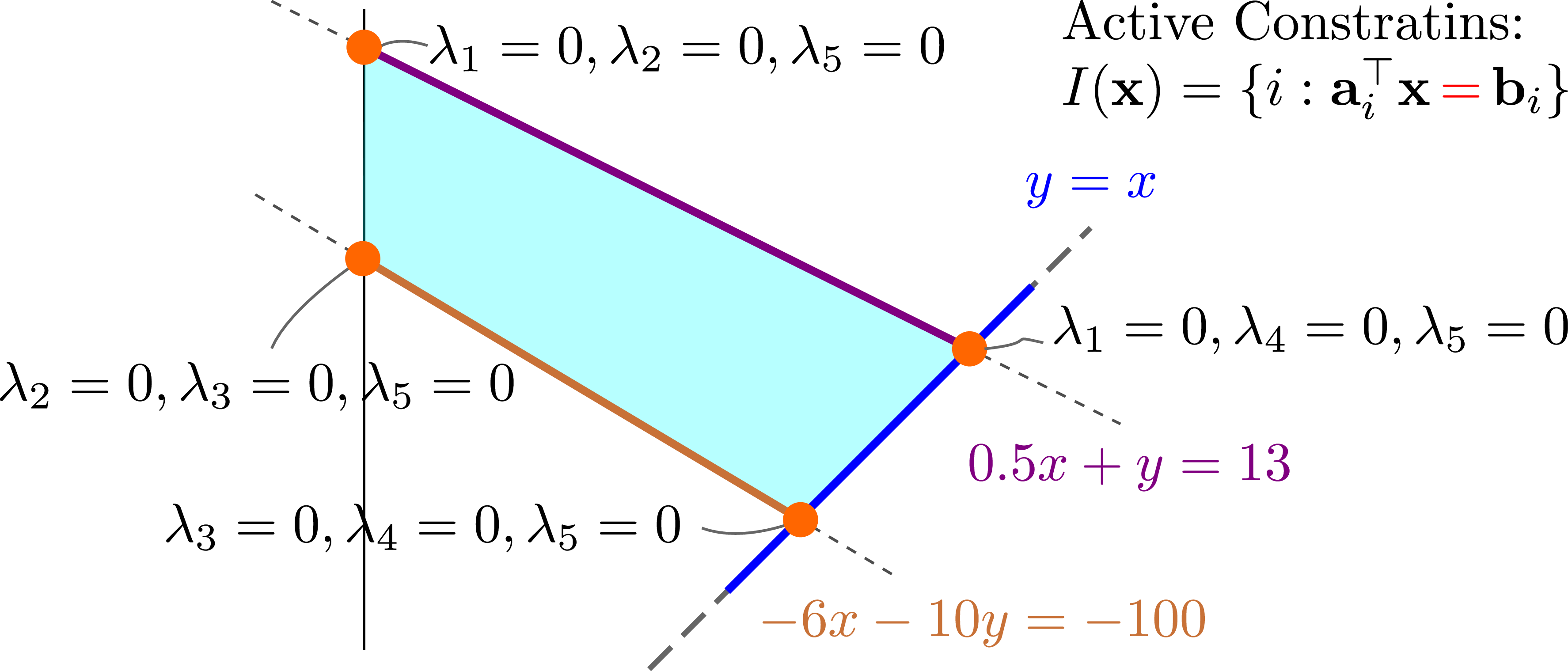
Active constraints
The constraint is active or binding when at the optimal solution the constraint holds with equality '='.
Video Example#
Variables
\(x\), \(y\)
\(\lambda_1, \lambda_2, \lambda_3, \lambda_4, \lambda_5\)
Stationarity
Slackness
Feasibility
Optimality conditions#
Slackness
Optimal solution at \((x,y)=(0,10)\).
Active constraints for example#
Which of the constraints is active or binding at the optimal solution?
\(\lambda_i=0\) if \(i\) is not active.
Big picture#
Big picture view#