
Worksheet Chapter 8, Part 3#
Notebook Info#
Topics#
This section focuses on using CVXPY to actually solve convex optimization problems, largely running parallel to Chapters 8.4 of Beck. However, note that the textbook is based on CVX, which is similar to CVXPY but for matlab.
You will learn to:
Use CVXPY to solve convex optimization problems.
Test this on examples including Chebyshev center of points.
⚙️ Requirements#
You should already have CVXPY installed from previous lectures. If you have issues with installation, I STRONGLY recommend you do everything in this class inside of a conda environment; see this conda tutorial for additional details.
Additional resources#
import cvxpy as cp
%matplotlib inline
import matplotlib.pylab as plt
import numpy as np
from mpl_toolkits.mplot3d import Axes3D
Least squares#
Suppose we want to solve the least squares problem
where
A = np.array([[1, 2], [3, 4], [5, 6]])
b = np.array([7, 8, 9])
Notice that this is a case where there is a point \(\mathbf{x} = (x_1,x_2)\) that actually solves the equation \(\mathbf{Ax} = \mathbf{b}\), and so the objective function
will have a minimum value of 0. This can be seen in the following graph, since there is a point where all the constraints from the rows of \(\mathbf{Ax} = \mathbf{b}\) intersect.
x_1 = np.linspace(-7,-5, 200)
plt.plot(x_1, (7-x_1)/2, label='x_1+2x_2=7')
plt.plot(x_1, (8-3*x_1)/4, label='3x_1+4x_2=8')
plt.plot(x_1, (9-5*x_1)/6, label='5x_1+6x_2=9')
plt.xlabel('x_1')
plt.ylabel('x_2')
plt.legend();
❓❓❓ Question ❓❓❓: Based on the graph above, approximately what is the minimizer \(\mathbf{x} = (x_1,x_2)\) of the objective function \(f(\mathbf{x}) = \min \| \mathbf{Ax} = \mathbf{b}\|^2\)?
Your answer here
Now we will solve the problem using CVXPY.
❓❓❓ Question ❓❓❓: Set up your expression using cvxpy’s variables and the given numpy arrays. Does CVXPY register the function as convex?
# Your code here

# Set up your variable
# x = ??

# Set up your expression
# expr = ??
Once we have an expression, we need to tell CVXPY whether we want it to be maximized or minimized. In this example, we want to find the minimizer so this is done as follows.
objective = cp.Minimize(expr)
print(objective)
Finally, we set up a problem class. Nothing happens when the problem is initialized, we’ll need to solve the problem which will happen in a few cell blocks.
myProb = cp.Problem(objective)
myProb = cp.Problem(cp.Minimize(expr)) # This is the same thing
print(myProb)
If you haven’t yet solved the problem, the value of the variable \(x\) will be None as seen below where the x.value has no printout.
Note: If you have run later cells to solve the problem and then run this cell without restarting the kernel, it will already know what x should be and will print the solution value.
x.value
As promised, we run the solve command to actually find the minimizer. The printed value is the minimum value of the objective function found.
myProb.solve()
In order to see the value of the variables that achieves the optimum, that is now stored in the variable itself.
x.value
Finally, we can check this solution to see that plugging in the values gets us to nearly 0.
np.linalg.norm(A @ x.value - b)**2
The version where it doesn’t work#
We could have also tried to solve the problem by noting that
so we should get the same answer if we use the objective
❓❓❓ Question ❓❓❓:
Code in the expression using this other version. Does CVXPY register the expression as convex?
Then, use CVXPY to solve the optimization problem like above. What happens?
# Your code here
Introducing Constraints#
Now, we’d like to be able to not just optimize an objective function, but also place some restrictions on the \(\mathbf{x}\) input values that we will allow. To do this, we will use the following example problem.
❓❓❓ Question ❓❓❓: Our first problem is that if we code the objective function exactly as written, CVXPY will mark it as convex. So, you first notice that \(\sqrt{(x_1^2 + x_2^2 + 1)} = \|(x_1,x_2,1)\|\). Use this to write the expression so that CVXPY registers the function as convex.
# Your code here

x = cp.Variable(2)

# expr = ??
Now, we can encode the constraints. Each constraint is an equation involving our variables. For example, if we were constrained to the ball of radius 5, we could use the constraint below.
cp.norm(x) <= 5
Like the functions, CVXPY needs to register the constraints as resulting in a convex function also. In the example above, the expression is marked as convex. However, in the following expression where we are tryint to write the first constraint for our problem, \(|x_1| + |x_2| + \frac{x_1^2}{x_2} \leq 5\), CVXPY doesn’t realize this. We can check if the constraint satisfies the DCP (Disciplined Convex Programming) rules with cons.is_dcp().
cons1 = cp.abs(x[0]) + cp.abs(x[1])+ x[0]**2 / x[1]<= 5
print(f"cons1.is_dcp: {cons1.is_dcp()}")
Here is a graph of the region of interest.
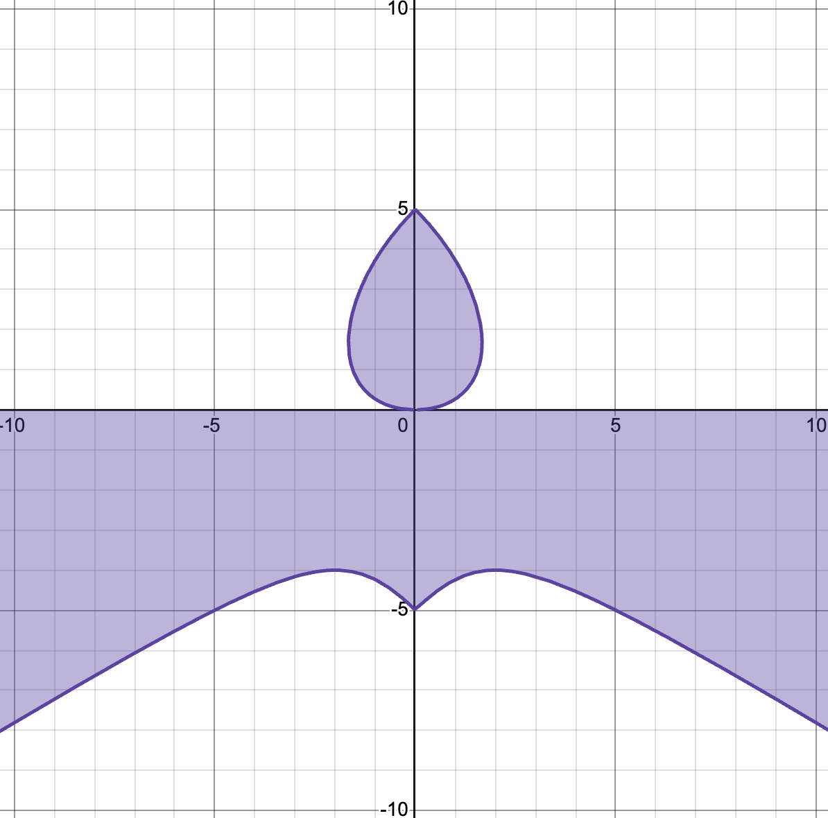
Notice that while the entire region is not convex, the additional restriction to \(x_2 \geq 0\) means the part we will actually work with (just the teardrop) will be convex. One way to handle this is with CVXPY’s quad_over_lin(Z,y) function (link to quad_over_lin documentation), which gives \((\sum_{i,j} Z_{i,j}^2)/y\), and is convex as long as \(y \geq 0\).
❓❓❓ Question ❓❓❓: fix the constraint below to use cp.quad_over_lin so that it registers as convex.
cons1 = cp.abs(x[0]) + cp.abs(x[1])+ x[0]**2 / x[1]<= 5
cons1.is_dcp()
The second constraint is
which also is not a convex set without some additional restriction.
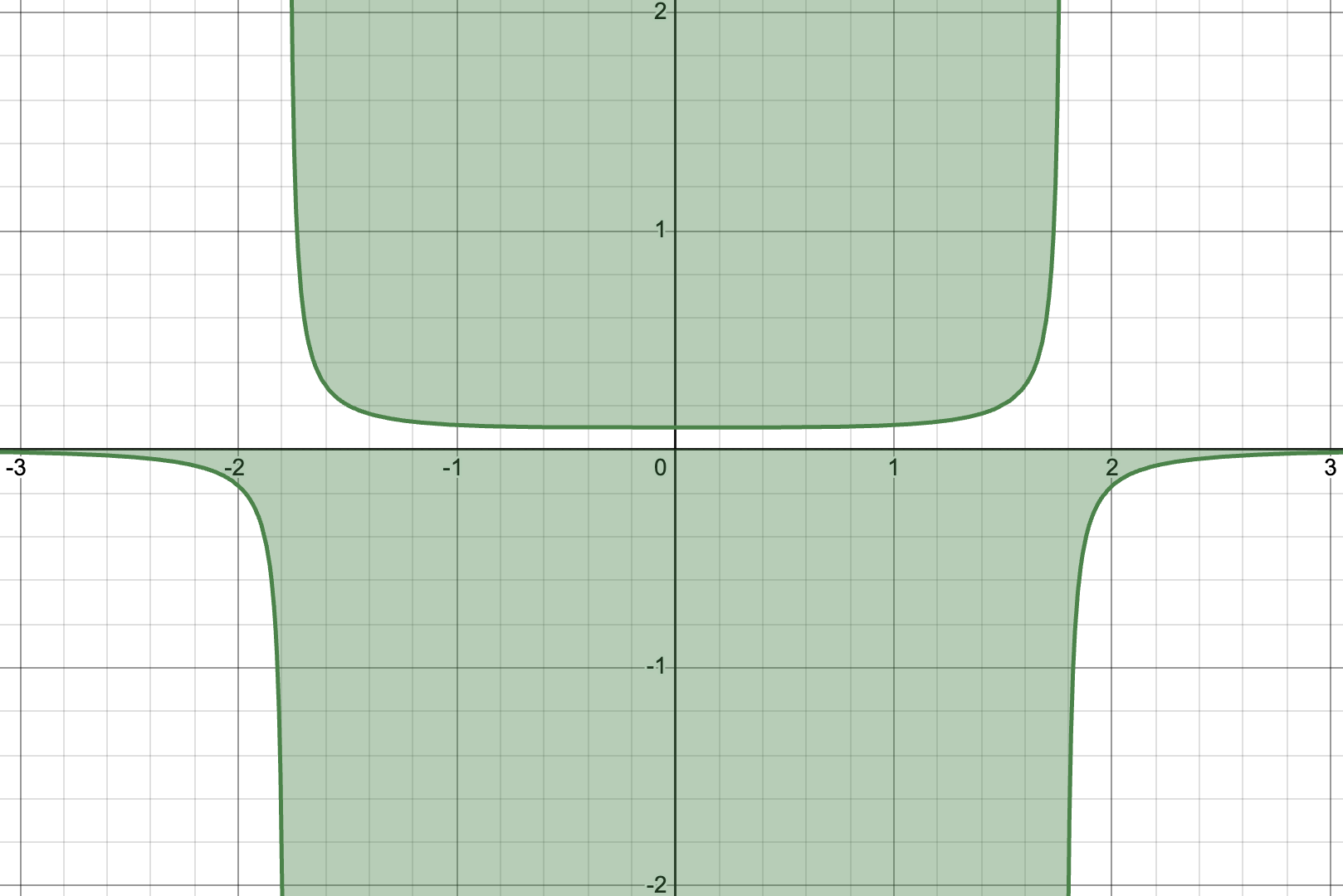
Below, we also see that coding the function as is does not register as convex in cvxpy.
cons2 = 1/x[1] + x[0]**4 <=10
print(f"cons2.is_dcp: {cons2.is_dcp()}")
But again, if we use the additional constraint that \(x_2\geq 0\) restriction, the part of the set that we care about is a convex set so we’re ok.
❓❓❓ Question ❓❓❓:
Fix cons2 using the cp.inv_pos function so that it registers as convex.
cons2 = 1/x[1] + x[0]**4 <=10
print(f"cons2.is_dcp: {cons2.is_dcp()}")
❓❓❓ Question ❓❓❓: The input to the cvxpy problem needs to be a list of all the constraints. Add the remaining ones to the list so that you have all 4 included.
myConstraints = [cons1, cons2, ] # Add the rest to the list
Once we have these constraints, we set up the problem with the constraints passed in as the second entry. Note that if the constraints do not satisfy the DCP condition, this will throw an error.
myProb = cp.Problem(cp.Minimize(expr3), myConstraints)
myProb.solve()
❓❓❓ Question ❓❓❓: What point \(\mathbf{x}\) minimizes the function?
# Your code here
Linear programming example#
From worksheet 8-1, we looked at the following problem.
❓❓❓ Question ❓❓❓: Use CVXPY to find the maximizer.
# Your code here
Chebyshev Center of Points#
Consider a collection of points \(\mathbf{a}_1, \mathbf{a}_2, \ldots, \mathbf{a}_m\) in \(\mathbb{R}^n\). The Chebyshev center is the center of the minimum radius closed ball containing all of the points.
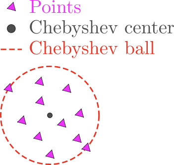
We want to find the center point, so we’ll call that point \(\mathbf{x}\). If the radius of the ball is \(r\), we know that all of the points are inside of the ball if
for each \(i = 1, \ldots, m\).
So, the full minimization problem is
Below, I have generated a matrix of data points in \(\mathbb{R}^2\).
A = np.random.normal(size=(100, 2), loc = (3,2))
plt.scatter(A[:, 0], A[:, 1])
plt.axis('square')
plt.show();
❓❓❓ Question ❓❓❓: Below is code to compute the smallest radius \(r\) that will enclose the points. Pick some different values for \(\mathbf{x}\), approximately where do you find the value to be the smallest?
x = np.array([4,3]) # <--- mess with this
r = max(np.linalg.norm(x - A[i, :]) for i in range(A.shape[0]))


plt.scatter(A[:, 0], A[:, 1], label = 'Data points')
plt.scatter(x[0], x[1], color='red', marker = '*',  label='Center')
# plot the circle of radius r around the center x
circle = plt.Circle((x[0], x[1]), r, color='blue', fill=False, label='Circle of radius r')
plt.gca().add_patch(circle)
plt.xlabel('x[0]')
plt.ylabel('x[1]')
plt.axis('square')
plt.title(f"Radius: {np.round(r,2)}")
plt.legend();
❓❓❓ Question ❓❓❓: Now, use CVXPY to solve for the optimum center based on your input data. Did you get a \(\mathbf{x}\) close to your guess above?
# Your code here
© Copyright 2025, The Department of Computational Mathematics, Science and Engineering at Michigan State University.