
Worksheet 11-2: The KKT Conditions (with Solutions)#
Download: CMSE382-WS11_2.pdf, CMSE382-WS11_2-Soln.pdf
Warning
This is an AI-generated transcript of the worksheet and may contain errors or inaccuracies. Please refer to the original course materials for authoritative content.
Worksheet 11-2: Q1#
Consider the problem
What are the function(s) \(g_i\) for this problem in Slater’s condition?
Solution
The functions \(g_i\) are the left-hand sides of the inequality constraints, so we have:
For each of the following, does the shown \(\hat{\mathbf{x}}\) satisfy Slater’s condition?
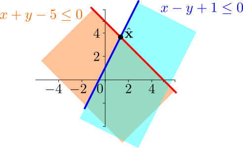
Solution
Slater’s condition requires that \(\hat{\mathbf{x}}\) must satisfy \(g_i(\hat{\mathbf{x}}) < 0\) for all \(i\). In the picture, this means it does not lie on the boundary where \(g_i(\hat{\mathbf{x}}) = 0\). Here, \(\hat{\mathbf{x}}\) lies on the boundary, so it does not satisfy Slater’s condition.
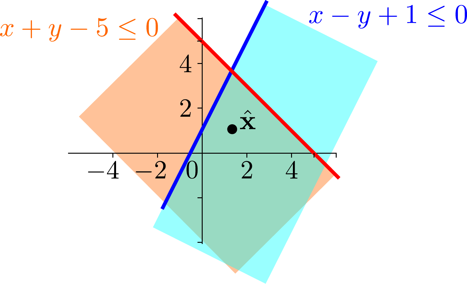
Solution
In this case, \(\hat{\mathbf{x}}\) lies in the interior of the feasible region, meaning that \(g_i(\hat{\mathbf{x}}) < 0\) for all \(i\), so it does satisfy Slater’s condition.
Worksheet 11-2: Q2#
Consider the same problem
What are the function(s) \(g_i\), \(h_j\), and \(s_k\) in the generalized Slater’s condition for this problem?
Solution
The inequality constraints are all affine, so the functions \(h_i\) are the left-hand sides of the inequality constraints, so we have:
For each of the following, does the shown \(\hat{\mathbf{x}}\) satisfy the generalized Slater’s condition?
Solution
Generalized Slater’s condition requires that \(\hat{\mathbf{x}}\) must satisfy \(g_i(\hat{\mathbf{x}}) < 0\) for all \(i\), however the affine \(h_j(\hat{\mathbf{x}})\) can be on the boundary. So, even though \(\hat{\mathbf{x}}\) lies on the boundary, it still satisfies the generalized Slater’s condition since the constraints are affine.
Solution
This is a bit of a trick question, but since the generalized Slater’s condition only requires that \(g_i(\hat{\mathbf{x}}) < 0\) for all \(i\), and there are no \(g_i\) in this problem, then \(\hat{\mathbf{x}}\) satisfies the generalized Slater’s condition regardless of where it is.
Worksheet 11-2: Q3#
Consider the problem
What are the function(s) \(g_i\), \(h_j\), and \(s_k\) in the generalized Slater’s condition for this problem?
Solution
The inequality constraints are all affine, so the functions \(h_i\) are the left-hand sides of the inequality constraints, so we have:
The equality constraint is also affine, so the function \(s_1\) is the left-hand side of the equality constraint, so we have:
For the following, does the shown \(\hat{\mathbf{x}}\) satisfy the generalized Slater conditions?
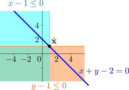
Solution
As in the last problem, the generalized Slater’s condition only requires that \(g_i(\hat{\mathbf{x}}) < 0\) for all \(i\), however the affine \(h_j(\hat{\mathbf{x}})\) and \(s_k(\hat{\mathbf{x}})\) can be on the boundary. There are no \(g_i\) in this problem, so \(\hat{\mathbf{x}}\) satisfies the generalized Slater’s condition regardless of where it is.
Worksheet 11-2: Q4#
For each of the following problems, draft a solution strategy for obtaining the optimal solution, if it exists. That is, describe the steps you would take to solve the problem without actually solving, with a particular focus on whether the KKT conditions are necessary and/or sufficient for optimality, and if so, how you would use them to find the optimal solution.
\(\min{x_1^2-x_2}\) s.t. \(x_2=0\).
Solution
This is a linearly constrained, convex problem. That means the KKT conditions are necessary and sufficient for optimality. This can also be seen in this portion of the flow chart.
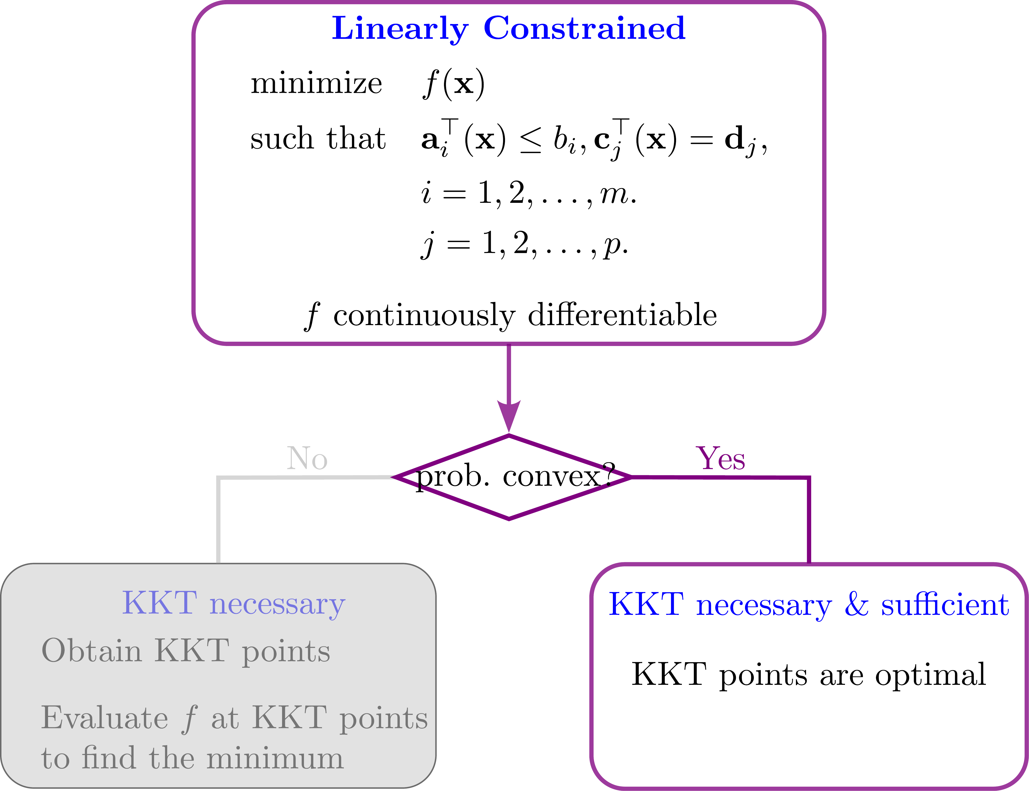
To solve this, we would first write down the Lagrangian, then compute the gradient of the Lagrangian with respect to \(\mathbf{x}\) and set it equal to zero. This will give us a system of equations, which we can solve to find the optimal solution.
\(\min{x_1^2-x_2}\) s.t. \(x_2^2 \leq 0\).
Solution
This is an inequality and equality constrained problem, although there are no equality constraints. It is a convex problem since the objective function is convex (check the Hessian) and the inequality constraint is convex (again check the Hessian). So, this means that the KKT conditions are sufficient for optimality, meaning if we have a KKT point, then it is an optimal solution.
To determine if the KKT conditions are necessary, we need to check if Slater’s condition is satisfied. To solve this, we would first check if there are any feasible points that satisfy the constraint \(x_2^2 \leq 0\) but \(x_2^2<0\). Any point that satisfies this constraint is of the form \((x_1,0)\), but this is on the boundary. So this does not satisfy Slater’s condition, and thus the KKT are not necessary for optimality. This means that the optimal solutions are not guaranteed to satisfy the KKT conditions.
This can also be seen in this portion of the flow chart:
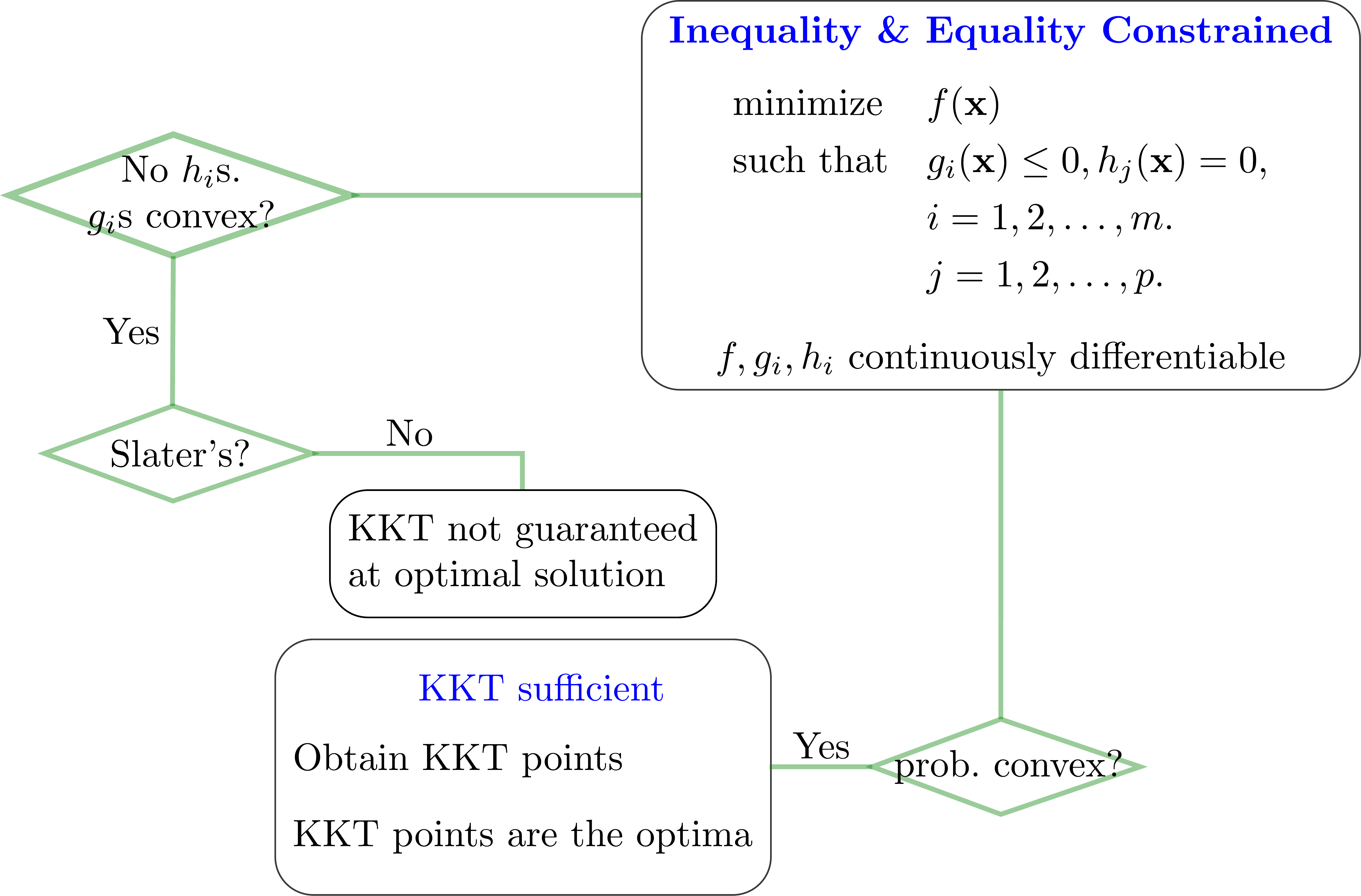
Note that this problem has the same result as the previous question since \(x_2^2 \leq 0\) implies \(x_2=0\), so the feasible region is the same as in the previous problem, and thus the best solution strategy is to replace the constraint with \(x_2=0\) and solve the convex problem.
Worksheet 11-2: Q5#
Consider the problem
Does this problem satisfy Slater’s condition?
Solution
The function \(g_1(\mathbf{x}) = 2x_1 + x_2 - 1\) is affine, so it is convex. The function \(g_2(\mathbf{x}) = x_1^2 - 1\) is convex since it is a quadratic with positive leading coefficient. The point \(\hat{\mathbf{x}} = (0,0)\) satisfies \(g_1(\hat{\mathbf{x}}) = -1 < 0\) and \(g_2(\hat{\mathbf{x}}) = -1 < 0\), so \(\hat{\mathbf{x}}\) satisfies Slater’s condition.
Are the KKT conditions necessary for optimality for this problem? Are the KKT conditions sufficient for optimality for this problem?
Solution
Since the problem satisfies Slater’s condition, the KKT conditions are necessary. Since the problem is convex, the KKT conditions are also sufficient.
Time permitting, solve the problem using the KKT conditions. Hint: Check the case where \(\lambda_1 > 0\) and \(\lambda_2 = 0\) first, where \(\lambda_1\) is associated to the \(2x_1+x_2=1\) constraint and \(\lambda_2\) is associated to the \(x_1^2=1\) constraint.
Solution
The Lagrangian for this problem is
so the KKT conditions are
As in previous worksheets, we solve this by checking the possible cases in terms of which constraints are active.
We get lucky and happen to check the case where \(\lambda_1 > 0\) and \(\lambda_2 = 0\) first. Because \(\lambda_1(2x_1 + x_2 - 1) = 0\), we have \(2x_1 + x_2 - 1 = 0\). Now we have three equations and three unknowns,
After some obnoxious algebra, we can solve this system to get \(x_1 = \frac{1}{16}\), \(x_2 = \frac{7}{8}\), and \(\lambda_1 = \frac{1}{4}\). So, \((\frac{1}{16}, \frac{7}{8})\) is a KKT point. From everything we did above, we know that the KKT conditions are necessary and sufficient for optimality, so this is the optimal solution to the problem.
This means we don’t actually have to check the rest of the conditions, but here are the other options for completeness.
If \(\lambda_1 = 0\) and \(\lambda_2 = 0\), then by the stationarity conditions, we have \(8x_1 - 1 = 0\) and \(2x_2 - 2 = 0\), so \(x_1 = \frac{1}{8}\) and \(x_2 = 1\). This does not satisfy the constraint \(2x_1 + x_2 - 1 \leq 0\), so this is not a KKT point.
If \(\lambda_1 >0\) and \(\lambda_2>0\), then by the slackness condiions, we have \(2x_1 + x_2 - 1 = 0\) and \(x_1^2 - 1 = 0\). These can be solved to get \(x_1 = \pm 1\) and \(x_2 = 1 - 2x_1\), meaning the possible points are \((-1,3)\) and \((1,-1)\).
For \((1,-1)\), the first stationarity condition gives \(7 + 2\lambda_1 + 2\lambda_2 = 0\), which is impossible because you can’t add positive numbers (\(\lambda_1\) and \(\lambda_2\)) to a positive number (7) and get 0. Thus, \((1,-1)\) does not satisfy the KKT conditions.
For \((-1,3)\), the second stationarity condition becomes \(4 + \lambda_1 = 0\), which is also impossible since \(\lambda_1\) is positive. Thus, \((-1,3)\) also does not satisfy the KKT conditions.
If \(\lambda_1 = 0\) and \(\lambda_2 > 0\), then because \(\lambda_2(x_1^2 - 1) = 0\), we have \(x_1^2 - 1 = 0\). This means \(x_1 = \pm 1\). By the second stationarity condition, we have \(2x_2 - 2 + \lambda_1 = 0\), so \(x_2 = 1\). This gives us the options \((1,1)\) and \((-1,1)\).
For \((1,1)\), the first constraint \(2x_1 + x_2 - 1 \leq 0\) is not satisfied, so this is not a KKT point.
For \((-1,1)\), the first stationarity condition gives \(-9-2\lambda_2 = 0\), which is impossible since \(\lambda_2\) is positive. Thus, \((-1,1)\) also does not satisfy the KKT conditions.
The only KKT point we found was \((\frac{1}{16}, \frac{7}{8})\), and since the KKT conditions are necessary and sufficient for optimality, this is the optimal solution to the problem.