Homework 5#
Note
This homework is due Friday, April 10, 11:59pm on Crowdmark. No credit will be given after Sunday, April 12, 11:59pm.
Instructions#
Problems are worth points as noted. You may receive partial credit for correct work leading to a solution. Note you will upload solutions for each question individually to Crowdmark. This can either be handwritten or typed, but make sure your work is clear and legible.
You will also enter information about what resources you used to complete the homework (e.g., textbook, lecture notes, online resources, generative AI, study groups, etc.) when you upload your solutions to Crowdmark.
import numpy as np
import matplotlib.pyplot as plt
Problem 1#
Consider the problem
a. Is this problem convex?
b. List the KKT conditions of the problem. Make sure to include all conditions, including conditions on \(\lambda\), and the constraints of the problem itself.
c. (Optional for extra practice: do NOT upload part (c). It will not be graded): Solve the problem and comment on whether the optimal solution (if it exists) is local or global.
Problem 2#
Consider the problem
Is this problem convex?
This problem has a solution since it consists of minimizing a continuous function over a nonempty compact set. Find an optimal solution. Remember to consider two cases of \(\lambda\): \(\lambda>0\) and \(\lambda=0\).
Problem 3 (Coding Problem)#
Consider \(\mathbf{a}_1, \ldots, \mathbf{a}_m \in \mathbb{R}^n\). For a given \(\mathbf{x} \in \mathbb{R}^n\backslash \{0\}\) and \(y \in \mathbb{R}\), define the hyperplane \(H_{\mathbf{x},y} = \{\mathbf{a} \in \mathbf{R}^n: \mathbf{x}^{\top} \mathbf{a}=y\}.\)

The orthogonal regression problem seeks to find a nonzero vector \(\mathbf{x} \in \mathbb{R}^n\) and \(y \in \mathbb{R}\) such that the sum of the squared Euclidean distances between \(\mathbf{a}_1, \ldots, \mathbf{a}_m\) to \(H_{\mathbf{x},y}\) is minimal, i.e., it is the solution to the problem
where \(d(\mathbf{a}_i,H_{\mathbf{x},y})\) is the distance function from point \(\mathbf{a}_i\) to hyperplane \(H_{\mathbf{x},y}\).
Let \(\mathbf{a}_1, \ldots, \mathbf{a}_m \in \mathbb{R}^n\) and let \(A\) be the matrix given by
An optimal solution of the orthogonal regression problem is the hyperplane \(H_{\mathbf{x},y}\) where \(\mathbf{x}\) is given by the eigenvector of the matrix
associated with the minimum eigenvalue, and the scalar is given by
where \(\mathbf{e}\) is a vector of ones of length \(m\).
For this problem, do the following:#
Watch the Orthogonal regression video, which covers the content written above.
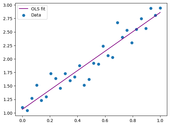
Copy the code in the cell below to generate a small data set. Note that this also draws the standard Ordinary Least Squares (OLS) line.
Determine the orthogonal regression fit by coding the solution directly from the discussion above:
Construct the matrix \(A\) from the given
data_xanddata_yWrite code to build the matrix \(A^{\top}(I_m-\frac{1}{m}\mathbf{e}\mathbf{e}^{\top})A\).
Obtain the minimum eigenvalue for that matrix and the corresponding eigenvector.
Plot the orthogonal regression fit based on the eigenvector you found.
Upload a pdf to Crowdmark that contains the following as the solution to this problem:
The code you used to compute the orthogonal regression line.
A plot of the orthogonal regression line found on top of the OLS and data plot from the code.
A table that gives the equation of both the OLS and the orthogonal regression lines found above.
A paragraph comparing the quality of fit for each method.
import matplotlib.pylab as plt
import numpy as np

# Generate synthetic data
np.random.seed(42)
data_x = np.linspace(0, 1, 30)
data_y = 2*data_x + 1 + 0.2 * np.random.randn(30)

# Obtain OLS fit and plot it
A_ols = np.array([np.ones(30), data_x]).T
x_ls = np.linalg.lstsq(A_ols, data_y, rcond=None)[0]

plt.plot(data_x, A_ols@x_ls, label='OLS fit', color='purple')
plt.scatter(data_x, data_y, label='Data');
plt.legend();