
Lecture 9-1: Optimization over a Convex Set#
Download the original slides: CMSE382-Lec9_1.pdf
Warning
This is an AI-generated transcript of the lecture slides and may contain errors or inaccuracies. Please refer to the original course materials for authoritative content.
This Lecture#
Topics:
Stationarity
Stationarity in convex problems
Orthogonal projection revisited
Gradient projection method
Announcements:
Homework 4 due TODAY.
Stationarity#
Recall: Stationary point of a function in unconstrained optimization#
Consider the unconstrained optimization problem
Definition (Stationary point of a function)
Let \(f: U \to \mathbb{R}\) be a function defined on a set \(U\subseteq \mathbb{R}^n\). Suppose that \(\mathbf{x}^* \in \text{int}(U)\) and that \(f\) is differentiable over some neighborhood of \(\mathbf{x}^*\). Then \(\mathbf{x}^*\) is called a stationary point of \(f\) if \(\nabla f(\mathbf{x}^*)=\mathbf{0}\).
It is a point where the gradient vanishes.
Stationary point of a function versus stationary point of a problem#
Stationary point of a problem in constrained optimization#
Consider the constrained optimization problem \((P)\):
Definition (Stationarity condition for a problem)
Let \(f\) be a continuously differentiable function over a closed convex set \(C\). Then \(\mathbf{x}^* \in C\) is called a stationary point of \((P)\) if
for any \(\mathbf{x} \in C\).
A point where there are no feasible descent directions.
Theorem (Stationarity as a necessary optimality condition)
Let \(f\) be a continuously differentiable function over a closed convex set \(C\), and let \(\mathbf{x}^*\) be a local minimum of \((P)\). Then \(\mathbf{x}^*\) is a stationary point of \((P)\).
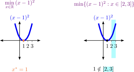
Equivalence of stationarity definitions when \(C=\mathbb{R}^n\)#
Consider
Stationary points for the problem satisfy
Choose \(\mathbf{x}=\mathbf{x}^* - \nabla f(\mathbf{x}^*)\):
But \(-\|\cdot\|^2 \leq 0\), so \(\nabla f(\mathbf{x}^*) = \mathbf{0}\).
Stationarity definitions for a constrained minimization problem and an unconstrained problem coincide when the feasible region becomes \(\mathbb{R}^n\).
Some special cases#
Feasible set |
Explicit stationarity condition |
|---|---|
\(C = \mathbb{R}^n\) |
\(\nabla f(\mathbf{x}^*) = \mathbf{0}\) |
\(C = \mathbb{R}^n_{+}\) |
\(\begin{cases} \frac{\partial f}{\partial x_i}(\mathbf{x}^*) = 0, & x_i^* > 0 \\ \frac{\partial f}{\partial x_i}(\mathbf{x}^*) \geq 0, & x_i^* = 0 \end{cases}\) |
\(\{\mathbf{x} \in \mathbb{R}^n : \mathbf{e}^{\top}\mathbf{x} = 1\}\) |
\(\frac{\partial f}{\partial x_1}(\mathbf{x}^*) = \ldots = \frac{\partial f}{\partial x_n}(\mathbf{x}^*)\) |
\(B[0,1]\) |
\(\nabla f(\mathbf{x}^*) = \mathbf{0}\) or \(|\mathbf{x}^*|=1\) and \(\exists \lambda \leq 0: \nabla f(\mathbf{x}^*)=\lambda \mathbf{x}^*\) |
Stationarity in Convex Problems#
Stationary point of a convex problem in constrained optimization#
Consider
where \(C\) is convex.
Theorem (Stationarity as a necessary optimality condition)
Let \(f\) be a continuously differentiable function over a closed convex set \(C\), and let \(\mathbf{x}^*\) be a local minimum of \((P)\). Then \(\mathbf{x}^*\) is a stationary point of \((P)\).
Theorem (Stationarity as necessary and sufficient condition for convex objective function)
Let \(f\) be a continuously differentiable convex function over a closed and convex set \(C \subseteq \mathbb{R}^n\). Then \(x^* \in C\) is a stationary point of \((P)\) if and only if \(x^*\) is an optimal solution of \((P)\).
Gradient Projection Method#
Recall: Orthogonal projection#
Definition (Orthogonal projection operator)
Given a nonempty closed convex set \(C\), the orthogonal projection operator \(P_C:\mathbb{R}^n \to C\) is defined by
Theorem (First projection theorem)
Let \(C\) be a nonempty closed convex set. Then the problem
has a unique optimal solution.
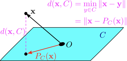
Returns the vector in \(C\) that is closest to input vector \(\mathbf{x}\).
Is a convex optimization problem:
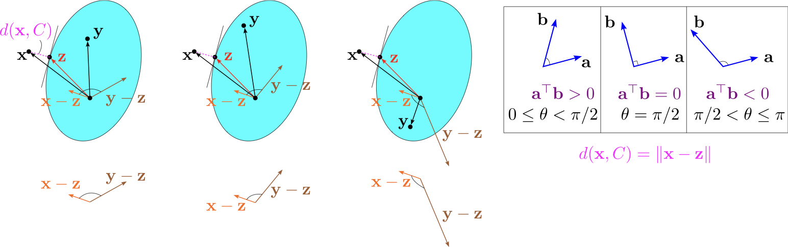
Orthogonal projection: Second projection theorem#
Theorem (Second projection theorem)
Let \(C\) be a closed convex set and let \(\mathbf{x} \in \mathbb{R}^n\). Then \(\mathbf{z} = P_C(\mathbf{x})\) if and only if \(\mathbf{z} \in C\) and
for any \(\mathbf{y} \in C\).
The angle between \(\mathbf{x} - P_C(\mathbf{x})\) and \(\mathbf{y} - P_C(\mathbf{x})\) is greater than or equal to \(90\) degrees.
Orthogonal projection: Non-expansiveness#
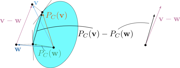
Theorem
Let \(C\) be a nonempty closed and convex set. Then
For any \(\mathbf{v},\mathbf{w} \in \mathbb{R}^n\), \((P_C(\mathbf{v})-P_C(\mathbf{w}))^{\top}(\mathbf{v}-\mathbf{w}) \geq \|P_C(\mathbf{v})-P_C(\mathbf{w})\|^2\).
(Non-expansiveness)
Representation of stationarity using the orthogonal projection operator#
Theorem (Stationarity in terms of the orthogonal projection operator)
Let \(f\) be a continuously differentiable function defined on the closed and convex set \(C\), and let \(s>0\). Then \(\mathbf{x}^* \in C\) is a stationary point of
if and only if
This leads to the gradient projection method for finding stationary points of optimization problems over convex sets.
Gradient projection algorithm#
Input: tolerance parameter \(\varepsilon > 0\).
Initialization: Pick \(\mathbf{x}_0 \in C\) arbitrarily.
For any \(k = 0, 1, 2, \ldots\) do:
Pick a stepsize \(t_k\) by a line search procedure. For example, using fixed step size, exact line search, or backtracking.
Set
If \(\|\mathbf{x}_k-\mathbf{x}_{k+1}\| \leq \varepsilon\), then stop and output \(\mathbf{x}_{k+1}\).
In the unconstrained case, this is the same as gradient descent.
There are convergence results.