
Lecture 4-1: Gradient Method: Part 1#
Download the original slides: CMSE382-Lec4_1.pdf
Warning
This is an AI-generated transcript of the lecture slides and may contain errors or inaccuracies. Please refer to the original course materials for authoritative content.
Descent Direction#
Topics Covered#
Topics:
Descent direction
Gradient descent algorithm
Announcements:
Quiz 2 on Wednesday, Feb 4
Office hours posted on course webpage
Descent Direction#
Analytical approach:
Goal: Solve \(\min\{f(\textbf{x}) \mid \textbf{x} \in \mathbb{R}^n\}\)
Set \(\nabla f(\mathbf{x}) = 0\) and find the stationary points \(\{\mathbf{x}^*\}_i\)
Test \(\nabla^2 f\) at each \(\mathbf{x}^*\) to identify local optima
Find any other potential global optima (e.g., boundary points)
What if that’s not an option?
For example, where is \(\nabla f(x,y,z) = \mathbf{0}\) for
(I don’t wanna….)
Idea: The Foggy Mountain Analogy#
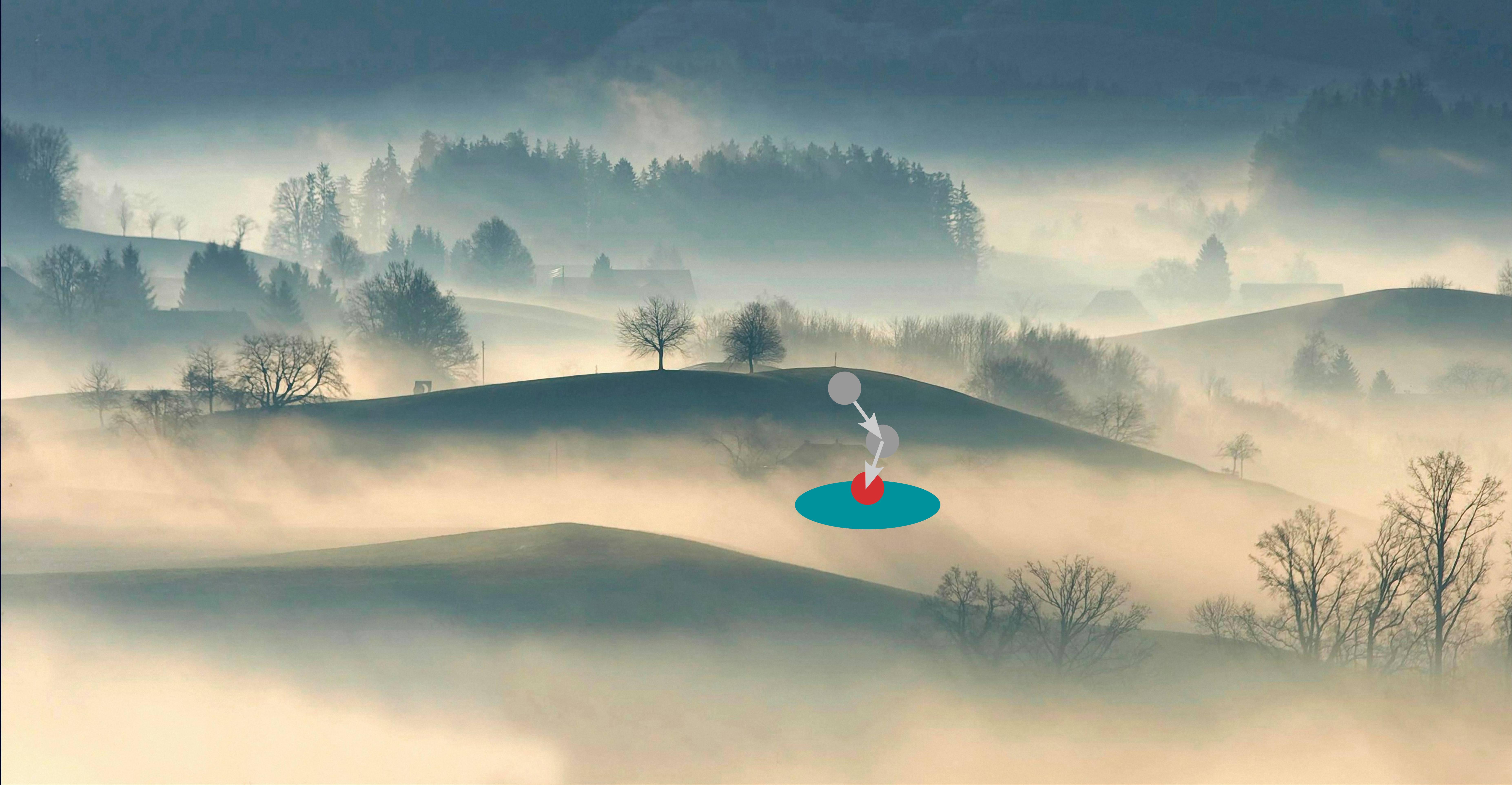
Photo by Ricardo Gomez Angel on Unsplash.
Descent Direction#
Given \(f:\mathbb{R}^n \to \mathbb{R}\) which is continuously differentiable.
Definition: The directional derivative of \(f\) at \(\mathbf{x}\) along the direction \(\mathbf{d}\) is defined as
Gives the instantaneous rate of change of \(f\) along direction \(\mathbf{d}\) through point \(\mathbf{x}\).
Definition: A nonzero vector \(\mathbf{d} \in \mathbb{R}^n\) is a descent direction of \(f\) at \(\textbf{x}\) if the directional derivative \(f'(\textbf{x};\textbf{d}) = \nabla f(\textbf{x})^\top \textbf{d}\) is negative.
Descent Direction (Lemma)#
Lemma: Let \(f\) be a continuously differentiable function over an open set \(U\), and let \(\textbf{x} \in U\). Suppose that \(\textbf{d}\) is a descent direction of \(f\) at \(\textbf{x}\).
Then there exists \(\varepsilon > 0\) such that
for any \(t \in (0, \varepsilon]\).
Translation: There is a \(t\) such that if you start at \(\textbf{x}\) and move along \(\textbf{d}\) for a distance \(t\), then you will reach a lower function value.
Gradient Descent Algorithm#
The foggy mountain: Using local information to navigate the global landscape
Decisions needed:
Starting point?
Descent direction?
In the gradient method \(\textbf{d}_k = -\nabla f (\textbf{x}_k)\).
Stepsize?
Stopping criteria?
Choosing the Stepsize#
Fixed step size keeps the step size constant.
How do we find the constant? Often heuristics, or trial and error.
Adaptive step size via exact line search for \(t_k\) that minimizes \(\min_{t\in \mathbb{R}} f(x_k +t \mathbf{d}_k)\).
Not always possible to find the exact minimizer.
Adaptive step size via backtracking line search: pick three parameters: an initial guess \(s > 0\), and \(\alpha \in (0, 1), \beta \in (0, 1)\). Then the stepsize is \(t_k = s\beta^{i_k}\), where \(i_k\) is the smallest non-negative integer such that \(f(\textbf{x}_k) - f(\textbf{x}_k + s\beta^{i_k}\textbf{d}_k) \geq -\alpha s\beta^{i_k} \nabla f(\textbf{x}_k)^\top\textbf{d}_k\).
Compromise that finds a “good enough” stepsize.
A theorem guarantees the existence of \(i_k\).
Annealing step size: Larger initial step size that is gradually decreased every step.
Steps are often exponentially decayed
Allows smaller steps as the algorithm approaches the minimum
The Gradient Method#
Input: tolerance parameter \(\varepsilon > 0\).
Initialization: Pick \(x_0 \in \mathbb{R}^n\) arbitrarily.
For any \(k = 0, 1, 2, \ldots\) do:
Set descent direction to \(\mathbf{d}=-\nabla f(\mathbf{x}_k)\)
Pick a stepsize \(t_k\)
For example, using exact line search on the function \(g(t) = f(\textbf{x}_k - t\nabla f(\textbf{x}_k))\).
Set \(\textbf{x}_{k+1} = \textbf{x}_k - t_k\nabla f(\textbf{x}_k)\).
If \(\|\nabla f(\textbf{x}_{k+1})\| \leq \varepsilon\), then STOP and \(\textbf{x}_{k+1}\) is the output.