
Lecture 3-1: Least Squares: Part 1#
Download the original slides: CMSE382-Lec3_1.pdf
Warning
This is an AI-generated transcript of the lecture slides and may contain errors or inaccuracies. Please refer to the original course materials for authoritative content.
Least Squares#
Topics Covered#
Ordinary Least Squares (OLS)
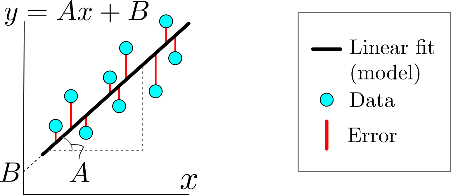
Linear fitting
Polynomial fitting
Overdetermined Systems#
Recall Matrix Rank
The rank of matrix \(A \in \mathbb{R}^{m\times n}\) is a non-negative integer \(\operatorname{rank}(A) \leq \max(m,n)\) given by any of the following:
the maximum number of its linearly independent rows or columns.
the number of non-zero rows in its row-echelon form
the number of non-zero singular values in its SVD
A linear system of the form \(\mathbf{A}\mathbf{x} = \mathbf{b}\), where \(\mathbf{A} \in \mathbb{R}^{m \times n}\) is of full rank and \(\mathbf{b} \in \mathbb{R}^m\) is
overdetermined if \(m>n\).
Almost always inconsistent (has no solution)
determined if \(m=n\), and the equations are independent
Has a unique solution
underdetermined if \(m<n\)
Either inconsistent (no solution), or infinitely many solutions
Goal: Obtain an approximate solution for overdetermined systems
Ordinary Least Squares Approximation#
Definition: The residual sum of squares error (or total sum of square errors) is
The minimizer of this equation is the least squares estimate
RSS measures how well \(\textbf{x}_{\text{LS}}\) approximates the data \(\mathbf{b}\)
The Least squares estimate minimizes \(\text{RSS}\):
You did this in CMSE381, but that textbook used the notation \(\beta_i\) for the coefficients. In this notation, the entries of \(\mathbf{x}\) are the coefficients of the linear function we’re trying to learn.
Linear Data Fitting#
Given a set of data points \((\mathbf{s}_i,t_i)\), \(i=1,2,\dots,m\), where \(\mathbf{s}_i\in\mathbb{R}^n\) and \(t_i\in\mathbb{R}\)
Assume that the target \(t_i\) can be approximated by the linear transformation of the data \(\mathbf{s}_i\):
Then the least squares method is applied to find the parameter \(\mathbf{x}\) that solves the following optimization problem:
Polynomial Fitting#
If we know that the points are approximately related to a polynomial of degree at most \(d\), i.e., there exists \(a_0, \ldots, a_d\) such that
we can use OLS \(\min\limits_{\textbf{x} \in \mathbb{R}^n}\|\mathbf{S}\textbf{x} - \mathbf{t}\|^2\) with
where