
Lecture 5-1: Newton Method: Part 1#
Download the original slides: CMSE382-Lec5_1.pdf
Warning
This is an AI-generated transcript of the lecture slides and may contain errors or inaccuracies. Please refer to the original course materials for authoritative content.
Review: Linear and Quadratic Approximation#
Topics Covered#
Topics:
Linear approximation theorem
Quadratic approximation theorem
Pure Newton’s method
Newton method quadratic local convergence
Announcements:
Homework 2 posted, due Thursday, Feb 12 at 11:59pm
Midterm 1 on Wednesday, Feb 18.
Linear Approximation Theorem#
Theorem (Linear Approximation Theorem):
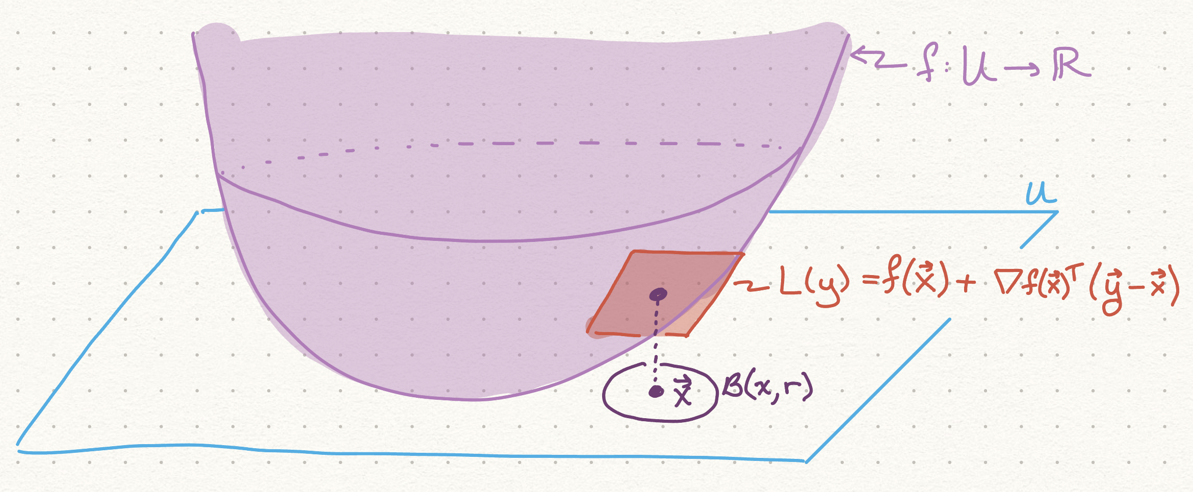
Let \(f : U \to \mathbb{R}\) be a twice continuously differentiable function over an open set \(U \subseteq \mathbb{R}^n\),
Let \(\mathbf{x} \in U\), \(r > 0\) satisfy \(B(\mathbf{x}, r) \subseteq U\).
Then for any \(\mathbf{y} \in B(\mathbf{x}, r)\) there exists \(\boldsymbol{\xi} \in [\mathbf{x}, \mathbf{y}]\) such that
Linear Approximation Visual#
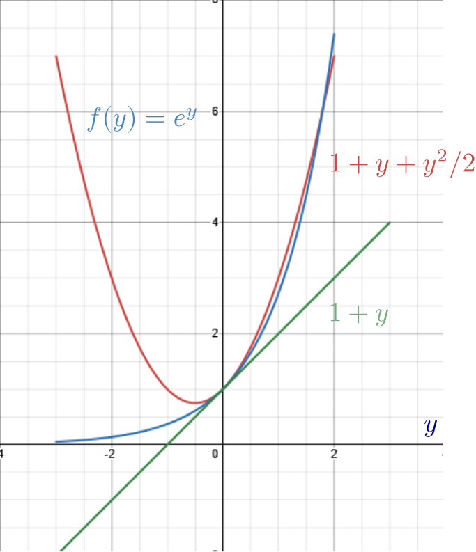
Quadratic Approximation Theorem#
Theorem (Quadratic Approximation Theorem):
Let \(f : U \to \mathbb{R}\) be a twice continuously differentiable function over an open set \(U \subseteq \mathbb{R}^n\).
Let \(\mathbf{x} \in U\), \(r > 0\) satisfy \(B(\mathbf{x}, r) \subseteq U\).
Then for any \(\mathbf{y} \in B(\mathbf{x}, r)\)
Newton’s Method#
Newton’s Method Introduction#
Newton’s method focuses on optimizing
where \(f\) is twice continuously differentiable.
Newton’s method is a second order method
Uses information from the Hessian
Contrast with first order methods like gradient descent which only uses gradient information
Requires that \(\nabla^2 f (\mathbf{x})\) is positive definite for every \(\mathbf{x} \in \mathbb{R}^n\)
A unique optimal solution \(\mathbf{x}^*\) exists.
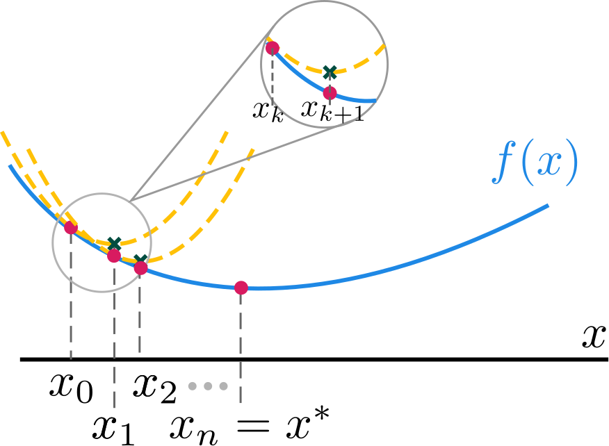
Newton’s Method - Main Idea#
Main idea: Minimize the quadratic approximation around \(\textbf{x}_k\):
This function is not well-defined unless \(\nabla^2f(\textbf{x}_k) \succ 0\).
The unique minimizer is the unique stationary point:
or equivalently \(\textbf{x}_{k+1} = \textbf{x}_k -(\nabla^2 f(\textbf{x}_k))^{-1}\nabla f(\textbf{x}_k)\)
\(-(\nabla^2f(\textbf{x}_k))^{-1}\nabla f(\textbf{x}_k)\) is called the Newton direction.
Pure Newton’s Method#
Input: \(\varepsilon > 0\) tolerance parameter
Initialization: Pick \(\textbf{x}_0 \in \mathbb{R}^n\) arbitrarily.
\(\mathbf{x}_0\) too far from \(\mathbf{x}^*\) can cause divergence.
General step: For any \(k = 0, 1, 2, \ldots\), do:
Compute the Newton direction \(\mathbf{d}_k\), which is the solution to the linear system \(\nabla^2 f(\textbf{x}_k)\mathbf{d}_k = -\nabla f(\textbf{x}_k)\)
More efficient than inverting \(\nabla^2 f(\mathbf{x}_k)\) in \(\mathbf{d}_k=-(\nabla^2f(\textbf{x}_k))^{-1}\nabla f(\textbf{x}_k)\)
Set \(\textbf{x}_{k+1} = \textbf{x}_k+\mathbf{d}_k\)
If \(\|\nabla f(\textbf{x}_{k+1})\| < \varepsilon\), stop and output \(\textbf{x}_{k+1}\).
Newton’s Method: Example#
Example: \(f(x,y) = \frac12(10x^2+y^2)+5\log(1+e^{-x-y})\)
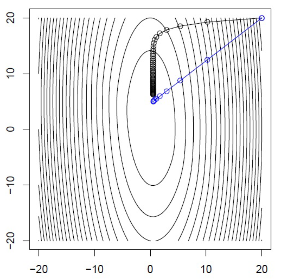
Comparison of Newton’s Method (blue) with Gradient Descent (black)
Convergence#
Quadratic Local Convergence of Newton’s Method#
Theorem: Let \(f\) be a twice continuously differentiable function defined over \(\mathbb{R}^n\). Let \(\{\textbf{x}_k\}_{k \geq 0}\) be the sequence generated by Newton’s method, and let \(\textbf{x}^\ast\) be the unique minimizer of \(f\) over \(\mathbb{R}^n\).
Assume that:
there exists \(m > 0\) such that \(\lambda_{\min}(\nabla^2 f(\textbf{x})) \geq m\) for any \(\mathbf{x} \in \mathbb{R}^n\)
there exists an \(L\) such that \(\nabla^2 f(\textbf{x})\) is Lipschitz with constant \(L\)
Then for any \(k = 0, 1, 2, \ldots\), the following inequality holds:
Moreover, if \(\|\textbf{x}_0-\textbf{x}^\ast \| \leq \frac{m}{L}\), then for \(k = 0, 1, 2, \ldots\):
Rapid convergence! (number of accuracy digits is doubled at each \(k\))
Can still converge if the assumptions are not met