Lecture 2-3: Optimality Conditions - Part 3

Download the original slides: CMSE382-Lec2_3.pdf

Warning

This is an AI-generated transcript of the lecture slides and may contain errors or inaccuracies. Please refer to the original course materials for authoritative content.

---

Global Optimality

Coercive Functions

Definition: A continuous function defined over \(\mathbb{R}^n\) is coercive if

\[\lim_{\|\mathbf{x}\|\rightarrow+\infty}f(\mathbf{x})=\infty.\]

Theorem: Let \(f \colon \mathbb{R}^n \to \mathbb{R}\) be a continuous and coercive function, and let \(S \subseteq \mathbb{R}^n\) be a closed set. Then \(f\) has a global minimum over \(S\).

Interactive example: desmos.com/3d/ajb6tdoryd

Quadratic Functions

Definition: A quadratic function over \(\mathbb{R}^n\) is a function of the form

\[f(\mathbf{x})=\mathbf{x}^\top\mathbf{A}\mathbf{x}+2\mathbf{b}^\top\mathbf{x}+c,\]

where \(\mathbf{A} \in \mathbb{R}^{n\times n}\) is symmetric, \(\mathbf{b} \in \mathbb{R}^n\), and \(c \in \mathbb{R}\).

For all \(\mathbf{x} \in \mathbb{R}^n\):

\[\nabla f(\mathbf{x}) = 2\mathbf{A}\mathbf{x}+2\mathbf{b}, \qquad \nabla^2 f(\mathbf{x}) = 2\mathbf{A}.\]

Example in \(\mathbb{R}^2\): Let \(\mathbf{A} = \begin{bmatrix} a_1 & a_2\\ a_2 & a_4 \end{bmatrix}\), \(\mathbf{b} = \begin{bmatrix} b_1 \\ b_2 \end{bmatrix}\), and \(c \in \mathbb{R}\). Then:

\[f(x_1, x_2) = a_1x_1^2+2a_2x_1x_2+a_4x_2^2+2b_1x_1+2b_2x_2+c.\]

Properties of Quadratic Functions

Let \(f(\mathbf{x})=\mathbf{x}^\top\mathbf{A}\mathbf{x}+2\mathbf{b}^\top\mathbf{x}+c\), where \(\mathbf{A} \in \mathbb{R}^{n\times n}\) is symmetric, \(\mathbf{b} \in \mathbb{R}^n\), and \(c \in \mathbb{R}\). Then:

a. \(\mathbf{x}\) is a stationary point of \(f\) if and only if \(\mathbf{A}\mathbf{x} = -\mathbf{b}\). b. If \(\mathbf{A} \succeq 0\), then \(\mathbf{x}\) is a global minimum point of \(f\) if and only if \(\mathbf{A}\mathbf{x} = -\mathbf{b}\). c. If \(\mathbf{A} \succ 0\) then \(\mathbf{x} = -\mathbf{A}^{-1}\mathbf{b}\) is a strict global minimum point of \(f\). d. \(f\) is coercive if and only if \(\mathbf{A} \succ 0\). e. \(f(\mathbf{x}) \geq 0\) if and only if \(\begin{bmatrix} \mathbf{A} & \mathbf{b} \\ \mathbf{b}^\top & c \end{bmatrix} \succeq 0\).

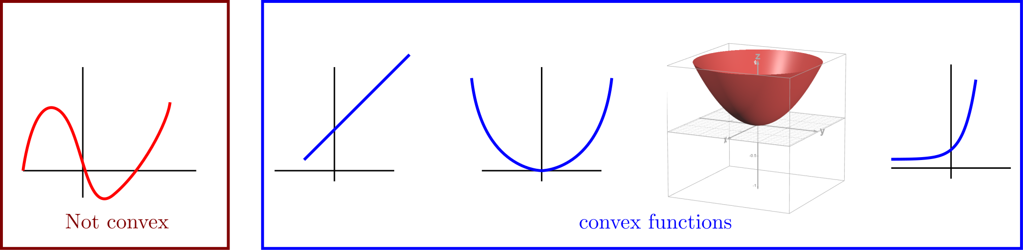
Convex Functions

Definition: Let \(f\) be a twice continuously differentiable function defined over \(\mathbb{R}^n\). If \(\nabla^2 f(\mathbf{x})\succeq \mathbf{0}\) for any \(\mathbf{x}\in\mathbb{R}^n\), we call the function convex (a generalization of “cup-shaped” real functions on \(\mathbb{R}\)).

Global Optima of Convex Functions

Theorem: Let \(f\) be a twice continuously differentiable function defined over \(\mathbb{R}^n\). Suppose that \(f\) is convex over its domain, i.e., \(\nabla^2f(\mathbf{x})\succeq \mathbf{0}\) for any \(\mathbf{x}\in\mathbb{R}^n\), and let \(\mathbf{x}^*\) be a stationary point of \(f\). Then:

• \(\mathbf{x}^*\) is a global minimum of \(f\).

• A local optimum of \(f\) is a global optimum.