
Worksheet Chapter 7, Part 2#
Topics#
This section focuses on using CVXPY to build convex functions using the tools we learned in the last class, largely focused on Chapters 7.1 to 7.4 of Beck. This notebook was developed in part using the following excellent tutorials:
You will learn to:
Set up expressions in CVXPY
Check if CVXPY registers them as convex
⚙️ Requirements#
Please ensure that you have cvxpy installed. We have had the best success with getting numpy upgraded first, but this is not a guarantee that it will work.
pip install --upgrade numpy
pip install cvxpy
Note that a very common issue is that numpy’s version doesn’t get updated with the installation of cvxpy and then causes havoc. I STRONGLY recommend you do everything in this class inside of a conda environment for this reason; see this conda tutorial for additional details.
import cvxpy as cp
%matplotlib inline
import matplotlib.pylab as plt
import numpy as np
from mpl_toolkits.mplot3d import Axes3D
Please note that some parts of this tutorial assume that you are working with CVXPY version \(\geq\) 1.1. Please check your version below.
print("cvxpy version:", cp.__version__)
cvxpy version: 1.8.1
Building Blocks#
Expressions in CVXPY are built from
variables; here we will use things like
x,y,z, etc.parameters; here we will use things like
a,b,c, etc.and constants, like Python floats or matrices.
Today’s notebook will focus on variables and constants.
Let’s start with single variables and parameters. The following code builds the expression
# Set our variable x and parameter a
x = cp.Variable()
a = cp.Parameter()

# define our expression

expr = 3.69 * x + 4 * a**2
Note that this looks like the computations we often do on regular floats or numpy arrays, however, this is actually storing the whole expression as a built in cvxpy class.
print(f"expr: {expr}")
print(f"type(expr): {type(expr)}")
expr: 3.69 * var1 + 4.0 * PowerApprox(param2, 2.0)
type(expr): <class 'cvxpy.atoms.affine.add_expr.AddExpression'>
In order to use more complex functions, we have a large assortment of atomic functions provided by cvxpy. So, if we want to encode the expression
we would do it as follows.
expr = cp.sqrt(1+cp.exp(x))
Notice that I had to use the cvxpy versions of functions, done by using cp.function since cvxpy was imported as cp above. Uncomment the following version where I put in numpy versions instead to see what happens.
# expr = np.sqrt(1+np.exp(x))
We can also make matrices of variables. For instance, if I want to encode the function
I can do it as follows.
X = cp.Variable((2,1)) #<--- note that I'm giving the variable a shape
A = np.array([[1,2],[3,4]])
b = np.array([[5],[6]])
expr = cp.norm(A@X - b, 2)
See the following for lists of atom functions:
❓❓❓ Question ❓❓❓:
Use CVXPY to encode the following expressions.
Throughout, save \(\mathbf{x} = (x_1,x_2)^\top\) as a \(2 \times 1\) variable, and assume
\(f_1(\mathbf{x}) = A\mathbf{x} - b\)
\(f_2(\mathbf{x})=\|A\mathbf{x}-b\|_2\)
\(f_3(\mathbf{x}) = \max \left( \|\mathbf{x}\|, \log(x_1)\right)\)
# Data
A = np.array([
    [-6.0, -10.0],
    [ 1.0,  -1.0],
    [ 0.5,   1.0],
    [-1.0,   0.0],
    [ 0.0,  -1.0]
])  # shape (5, 2)

b = np.array([
    [-100.0],
    [   0.0],
    [  13.0],
    [   0.0],
    [   0.0]
])  # shape (5, 1)

# Add your code here
Notice that these variables act like matrices. For instance, we can add and multiply them as long as the dimensions match:
# Now do example with higher dimensional variables
X = cp.Variable((2,2))
Y = cp.Variable((3,1))
Z = cp.Variable((2,2))

X+Z
Expression(AFFINE, UNKNOWN, (2, 2))
However, it will throw an error if their dimensions don’t match, just like if they were numpy matrices.
# Uncomment the line below to see the error.
# X+Y
In general, this code is built to look like numpy inputs. So as long as you remember that, for example, \(X\) is matrix of variables, then the commands from numpy will often work.
print("dimensions of X:", X.shape)
print("size of X:", X.size)
print("number of dimensions:", X.ndim)
print("dimensions of sum(X):", cp.sum(X).shape) #<-- this is a scalar, so it has shape ()
print("dimensions of A @ X:", (A @ X).shape)
dimensions of X: (2, 2)
size of X: 4
number of dimensions: 2
dimensions of sum(X): ()
dimensions of A @ X: (5, 2)
Sign#
For a lot of the functions, we will require either positive or negative inputs. This can be forced through though nonpos=True or nonneg=True flag for the cp.Variable class.
x = cp.Variable() #<-- this variable has no sign constraints, so it can be positive, negative, or zero
y = cp.Variable(nonpos=True) #<-- y <= 0
z = cp.Variable(nonneg=True) #<-- z >= 0


print("sign of x:", x.sign)
print("sign of y:", y.sign)
print("sign of z:", z.sign)
sign of x: UNKNOWN
sign of y: NONPOSITIVE
sign of z: NONNEGATIVE
We can also use this in expressions. For instance, even though we didn’t enforce positivity for x, we know that x**2 is always positive, as seen in the next line.
# Sign is determined from the input pieces of the expression, so we can check the sign of more complicated expressions.
c = np.array([1, -1])
print("sign of square(x):", cp.square(x).sign)
sign of square(x): NONNEGATIVE
❓❓❓ Question ❓❓❓:
The variables x, y, and z are saved below. Before writing code, determine which of the following expressions should be NONNEGATIVE, NONPOSITIVE, or UNKNOWN. Then write code to save each expression and check the sign using CVXPY.
\(f_1(x,y) = xy\)
\(f_2(z) = -z\)
\(f_3(x,y,z) = e^{x+y+z}\)
\(f_4(x, z) = \max\{x,z\}\)
\(f_5(x, y, z) = |x+y-z|\)
x = cp.Variable()
y = cp.Variable(nonpos=True) #<-- y <= 0
z = cp.Variable(nonneg=True) #<-- z >= 0


# Code your expressions here
Curvature#
Curvature is what CVXPY uses to describe the shape of the function. It can be checked with expr.curvature. The options for curvature (as of cvxpy version 1.1) are as follows:
convex
concave
affine
constant
quasiconvex
quasiconcave
quasilinear
unknown.
We’ve discussed convex extensively in class. A function \(f\) is concave if its negative \(-f\) is convex.
We’ll start by focusing on convex, concave, affine, constant, and unknown.
x = cp.Variable()
X = cp.Variable((2,1))
A = np.array([[1,2],[3,4]])
B = np.array([[5],[6]])

print(f"Constant function: {cp.Constant(5).curvature}")
print(f"||A @ X - B|| : {cp.norm(A @ X - B, 2).curvature}")
print(f"-x^2 : {(-cp.square(x)).curvature}")
print(f"A@X-B : {(A @ X - B).curvature}")
Constant function: CONSTANT
||A @ X - B|| : CONVEX
-x^2 : CONCAVE
A@X-B : AFFINE
When given a complex expression, the CVXPY code does exactly what we did in the last class and tries to determine if a new function is convex based on other ones.
Example#
Consider the function
t = np.linspace(-10, 10, 100)
plt.plot(t, 2*t**2 + 3)
plt.title("Plot of f(t) = 2t^2 + 3")
plt.show();
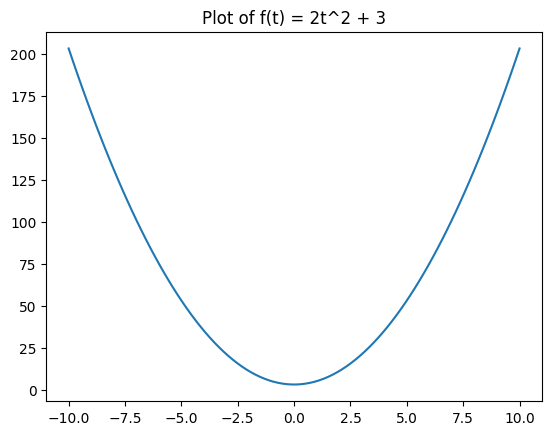
We can build the convexity of this function up from our rules from last class as follows:
\(x\) is an affine function (so it is also automatically convex)
\(x^2\) is a convex function because it is a quadratic function with a positive 2nd derivate (1-d verison of Hessian)
We can multiply a convex function by a positive constant to get a convex function, so \(2x^2\) is convex.
We can add a constant to a convex function to get a convex function, so \(2x^2 + 3\) is convex.
The logic for how CVXPY determines this is visualized in the following flow chart from cvxpy.org.
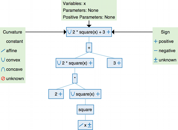
Note that this means that CVXPY might mark something as UNKNOWN even though the function is actually convex if it just can’t determine the convexity based on the rules above.
Quasiconvex and Quasiconcave#
A function \(f(\mathbf{x})\) is quasiconvex if its sublevelsets
are always convex sets.
Similarly, a function is quasiconcave if its superlevelsets
are always convex. Equivalently, a function is quasiconcave if \(-f\) is quasiconvex.
A quasiconvex example#
Now let’s think about the function
t = np.linspace(-10,10,100)
plt.plot(t, (1+t**2)**(1/2))
plt.title(r'$f(x) = \sqrt{1+x^2}$')
plt.show();
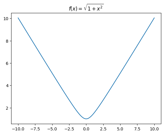
❓❓❓ Question ❓❓❓: Using the second derivative test, determine if this function is convex.
Your answer here
Click for solution
Note that we can’t just use the composition stuff:
We already established that \(x^2\) is convex
Add a constant to get that \(1+x^2\) is convex.
Note that \(\sqrt{\cdot}\) is concave, not convex, so we can’t just use the composition rule.
Instead, we use the second derivative test. For \(f(x) = \frac{x}{\sqrt{1+x^2}}\)
Since \(f''(x)>0\) for any input \(x\), the function is convex
❓❓❓ Question ❓❓❓: What does CVXPY think the curvature of \(f\) is?
# Your code here
x = cp.Variable()
f = cp.sqrt(1+cp.square(x))
print(f"f curvature: {f.curvature}")
print(f"f is convex: {f.is_convex()}")
f curvature: QUASICONVEX
f is convex: False
It turns out we can write the function a different way.
❓❓❓ Question ❓❓❓: Expand the function
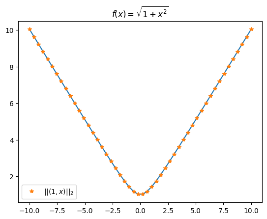
to double check that it is the same as \(f(x)\) above. The code below also plots this function so that we can see it is exactly the same.
Your notes here
Click for solution
\(g(x) = \|(1,x)\| = \sqrt{1^2 + x^2} = \sqrt{1 + x^2}\)
t = np.linspace(-10,10,50)
plt.plot(t, (1+t**2)**(1/2))
plt.plot(t, np.linalg.norm(np.vstack([t, np.ones_like(t)]), axis=0), marker = '*', linestyle = 'None', label = '$||(1,x)||_2$')
plt.title(r'$f(x) = \sqrt{1+x^2}$')
plt.legend()
plt.show();
❓❓❓ Question ❓❓❓: Code the expression for \(g\) in CVXPY and check it’s curvature. Is it the same as the curvature for \(f\)?
Hint: You’ll need the cp.hstack and cp.norm functions.
# Your code here
Click for solution
You should NOT have gotten the same output of curvature for \(f\) and \(g\) above. This is because CVXPY uses a system of rules to determine if something is convex. However, if this system of rules doesn’t promise convexity, it won’t say it’s convex. So you can interpret this as follows:
If CVXPY tells you a function is convex, it’s definitely convex.
If CVXPY tells you something else (in particular, “unknown”), that doesn’t mean the function is not convex… it just means that CVXPY couldn’t verify if it was.
In the case of the function above, it is in fact convex, but the format of \(f\) didn’t satisfy CVXPY’s checker when validating that, while the format of \(g\) did.
Quasilinear#
A function is quasilinear if it is BOTH quasiconvex and quasiconcave.
A Quasilinear example#
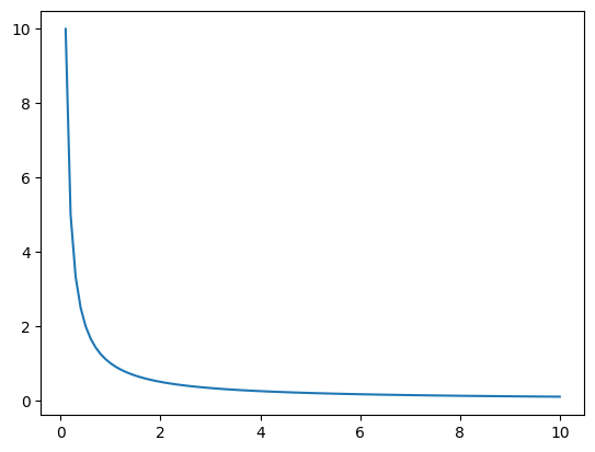
Let’s take a look at the function
for \(x >0\).
t = np.linspace(.1, 10, 100)
plt.plot(t, 1/t)
plt.show();
❓❓❓ Question ❓❓❓: Answer the following before coding anything.
Is \(f(x) = 1/x\) for \(x>0\) convex?
Is \(f(x) = 1/x\) for \(x>0\) concave?
Is \(f(x) = 1/x\) for \(x>0\) quasiconvex?
Is \(f(x) = 1/x\) for \(x>0\) quasiconcave?
Once you’ve done this by hand, write the expression in CVXPY and check the curvature.
Your notes here
Click for solution
The function is convex because the second derivative is \(f''(x) = 2x^{-3}\), which is always positive for positive \(x\).
The function is not concave since \(-f(x) = -\frac{1}{x}\), which has second derivative \(-2x^{-3}\) which is always negative. Since \(-f\) is not convex, \(f\) is not concave.
For any \(\alpha\), the sublevelset is \(\{x \mid 1/x \leq \alpha, x>0\} = \{x \mid x \geq 1/\alpha\}\) which is just an interval \([1/\alpha,\infty)\) which is convex. This means \(f(x)\) is quasiconvex.
For any \(\alpha\), the superlevelset (restricted to the domain \(x> 0\)) is \(\{x \mid 1/x \geq \alpha, x>0\} = \{x \mid 0< x \leq 1/\alpha\}\) which is just an interval \((0, 1/\alpha]\) which is convex. This means \(f(x)\) is quasiconcave.
Rules#
DCP rules (for CONSTANT, AFFINE, CONVEX, CONCAVE).
For DCP (Disciplined Convex Programming), the actual rules that CVXPY uses to determine the label are as follows.
\(f(\text{expr}_1, \text{expr}_2, ..., \text{expr}_n)\) is
CONVEXif \(f\) is a convex function and for each \(\text{expr}_{i}\) one of the following conditions holds:\(f\) is increasing in argument \(i\) and \(\text{expr}_{i}\) is convex.
\(f\) is decreasing in argument \(i\) and \(\text{expr}_{i}\) is concave.
\(\text{expr}_{i}\) is affine or constant.
\(f(\text{expr}_1, \text{expr}_2, ..., \text{expr}_n)\) is
CONCAVEif \(f\) is a concave function and for each \(\text{expr}_{i}\) one of the following conditions holds:\(f\) is increasing in argument \(i\) and \(\text{expr}_{i}\) is concave.
\(f\) is decreasing in argument \(i\) and \(\text{expr}_{i}\) is convex.
\(\text{expr}_{i}\) is affine or constant.
\(f(\text{expr}_1, \text{expr}_2, ..., \text{expr}_n)\) is
AFFINEif \(f\) is an affine function and each \(\text{expr}_{i}\) is affine.
If none of the three rules (convex, concave, affine) apply, the expression \(f(\text{expr}_1, \text{expr}_2, ..., \text{expr}_n)\) is marked as having UNKNOWN curvature under DCP.
DQCP extensions (for QUASICONVEX, QUASICONCAVE, QUASILINEAR). When DQCP (Disciplined Quasiconvex Programming) is enabled, CVXPY refines curvature further:
Any
CONVEXexpression is automaticallyQUASICONVEX, and anyCONCAVEexpression is automaticallyQUASICONCAVE.Certain additional “atoms” (e.g.,
length,ceil,floor,sign, some ratios and products) are known to be quasiconvex, quasiconcave, or both, so expressions built from them using the same kind of monotone/convex/concave/affine rules are labeled:QUASICONVEX(sublevel sets convex),QUASICONCAVE(superlevel sets convex), orQUASILINEAR(both quasiconvex and quasiconcave).
If none of the DCP or DQCP rules certify an expression, its curvature remains
UNKNOWN.
Extra Practice#
For each of the following functions, code the expression directly as written into cvxpy and see what its curvature is labeled as. Then see if you can find an equivalent forumlation of the function that results in the cvxpy registering the function as convex.
\(f_1(x,y) = \sqrt{x^2 + y^2}\)
\(f_2(x) = (x-1)(x-2)\)
\(f_3(x,y) = -\sqrt{xy}\)
# Your code here
© Copyright 2025, The Department of Computational Mathematics, Science and Engineering at Michigan State University.