Worksheet 3-1

Note

This jupyter notebook won’t run on the website. If you are viewing this online, click on the download (down arrow) button on the top right of the page, select the .ipynb option, and save the file locally. Then open it with your Jupyter system to edit the file.

✅ Put your name here.

✅ Put your group number here.

Topics covered

This notebook covers Chapter 3.1 and 3.2 from the textbook

• Overdetermined systems for least squares probelms

• Data fitting

• Curve fitting from least squares

%matplotlib inline
import matplotlib.pylab as plt
import numpy as np

Overdetermined systems

We are given a linear system of the form \(\mathbf{A}\mathbf{x}=\mathbf{b},\) where \(\mathbf{A}\in\mathbb{R}^{m\times n}\) and \(\mathbf{b}\in\mathbb{R}^m\).

• The system is overdetermined meaning that \(m>n\).

• In addition, we assume that \(\mathbf{A}\) has full column rank, i.e., \(\mathrm{rank}(\mathbf{A})=n\).

We will consider the linear system

\[\begin{split}\begin{align*} x_1+2x_2=&0,\\ 2x_1+x_2=&1,\\ 3x_1+2x_2=&1. \end{align*}\end{split}\]

which can be written in the form \(\mathbf{A}\mathbf{x}=\mathbf{b}\) as

\[\begin{split} \begin{bmatrix} 1 & 2\\ 2 & 1\\ 3 & 2 \end{bmatrix} \begin{bmatrix} x_1\\ x_2\\ x_3 \end{bmatrix} = \begin{bmatrix} 0\\ 1\\ 1 \end{bmatrix} \end{split}\]

A = np.array([[1, 2], [2, 1], [3, 2]])
b = np.array([0, 1, 1])

❓❓❓ Question ❓❓❓:

• What are \(m\) and \(n\) for this \(A\)? Save them below.

• What is the rank of the matrix? Use np.linalg.matrix_rank to determine this.

• Is the matrix full rank? That is, is the rank the same as min(m,n)?

• Is the matrix, overdetermined, determined, or underdetermined?

## Your answer here 

m = None 
n = None 

rk_A = None 

Show code cell content

Hide code cell content

### ANSWER 

m = A.shape[0]
n = A.shape[1]
rk_A = np.linalg.matrix_rank(A)

print("m =", m)
print("n =", n)
print("rank(A) =", rk_A)
print("\trank is the same as the minimum dimension, so it is full rank." )
print("Since m=3 is bigger than n=2 and A is full rank, A is overdetermined.")

m = 3
n = 2
rank(A) = 2
	rank is the same as the minimum dimension, so it is full rank.
Since m=3 is bigger than n=2 and A is full rank, A is overdetermined.

Solving the OLS problem

In general, when \(m>n\) and \(\mathrm{rank}(\mathbf{A})=𝑛\), we may not find a solution \(\mathbf{x}\) for the linear system (Why?). Instead, we try to find an approximate solution by optimizing

\[\min_{\mathbf{x}\in\mathbb{R}^{n}}\|\mathbf{A}\mathbf{x}-\mathbf{b}\|^2.\]

If there is a solution to the linear system, we will also find the solution by solving the optimization problem. So we will consider \(m\geq n\) in the rest of this lecture.

Let

\[f(\mathbf{x})=\|\mathbf{A}\mathbf{x}-\mathbf{b}\|^2.\]

We can expand this to see that

\[f(\mathbf{x})=\mathbf{x}^\top\mathbf{A}^\top\mathbf{A}\mathbf{x}-2\mathbf{b}^\top\mathbf{A}\mathbf{x}+\|\mathbf{b}\|^2.\]

❓❓❓ Question ❓❓❓: So that we don’t mix up \(A\)’s and \(b\)’s, I can write the quadratic form of a function as

\[ f(\mathbf{x}) = \mathbf{x}^\top \mathbf{Q} \mathbf{x} + 2 \mathbf{d}^\top \mathbf{x} + c \]

where \(\mathbf{Q}\) is symmetric.

What are \(\mathbf{Q}\) and \(\mathbf{d}\) for our function above? Check that \(Q\) is symmetric.

✎ Answer here.

Solution

• \(\mathbf{Q} = \mathbf{A}\mathbf{A}^\top\)

• \(\mathbf{d}^\top = -\mathbf{b}^\top \mathbf{A}\), so taking transposes we have \(\mathbf{d} = -\mathbf{A}^\top \mathbf{b}\).

Since we know that \(f\) is in quadratic form, we can use that quadratic functions have

\[ \nabla f(\mathbf{x}) = 2 \mathbf{Qx} + 2 \mathbf{d} \qquad \text{and} \qquad \nabla^2 f(\mathbf{x}) = 2 \mathbf{Q}. \]

to get

\[\nabla f(\mathbf{x}) = 2\mathbf{A}^\top\mathbf{A}\mathbf{x}-2\mathbf{A}^\top\mathbf{b}\]

and

\[\nabla^2f(\mathbf{x})=2\mathbf{A}^\top\mathbf{A}.\]

Because \(\mathbf{A}\) is of full column rank, we have \(\mathbf{A}^\top\mathbf{A}\) is positive definite. Therefore, by properties of quadratic functions from last class, the unique solution to the optimization problem \(\min_{\mathbf{x}\in\mathbb{R}^{n}}\|\mathbf{A}\mathbf{x}-\mathbf{b}\|^2\) is obtained at \(\mathbf{x} = \mathbf{Q}^{-1}\mathbf{d}\), which translates here to

\[ \mathbf{x}_{LS}=(\mathbf{A}^\top\mathbf{A})^{-1}\mathbf{A}^\top\mathbf{b}\]

This vector is called the least squares solution or the least squares estimate of the system \(\mathbf{A}\mathbf{x}=\mathbf{b}\).

We also write in the solution as

\[\mathbf{A}^\top\mathbf{A}\mathbf{x}_{LS}=\mathbf{A}^\top\mathbf{b},\]

which is called the normal system.

Example Let’s go back to the same example we were using above,

\[\begin{split} \begin{bmatrix} 1 & 2\\ 2 & 1\\ 3 & 2 \end{bmatrix} \begin{bmatrix} x_1\\ x_2\\ x_3 \end{bmatrix} = \begin{bmatrix} 0\\ 1\\ 1 \end{bmatrix} \end{split}\]

❓❓❓ Question ❓❓❓: Use numpy to find \(\mathbf{x}_{LS}=(\mathbf{A}^\top\mathbf{A})^{-1}\mathbf{A}^\top\mathbf{b}\).

## Your work here

A = np.array([[1, 2], [2, 1], [3, 2]])
b = np.array([0, 1, 1])

Show code cell content

Hide code cell content

### ANSWER  ####

A = np.array([[1, 2], [2, 1], [3, 2]])
b = np.array([0, 1, 1]).T

AtA = A.transpose()@A
Atb = A.transpose()@b

x_ls = np.linalg.inv(AtA)@Atb
print(x_ls)

[ 0.57692308 -0.30769231]

❓❓❓ Question ❓❓❓: Now use the numpy command np.linalg.lstsq to get (hopefully) the same answer.

# Uncomment the line below to show information about the lstsq function.
# ?np.linalg.lstsq

# Your answer here 

Show code cell content

Hide code cell content

### ANSWER 

np.linalg.lstsq(A, b)[0]

array([ 0.57692308, -0.30769231])

Show code cell content

Hide code cell content

#### ANSWER ####

x_ls2 = np.linalg.lstsq(A,b, rcond=None)[0]
print(x_ls2)
print(x_ls)

#Answer agrees.

[ 0.57692308 -0.30769231]
[ 0.57692308 -0.30769231]

Data Fitting

One application of least squares is data fitting. Suppose that we are given a set of data points \((\mathbf{s}_i,t_i)\), \(i=1,2,\dots,m\), where \(\mathbf{s}_i\in\mathbb{R}^n\) and \(t_i\in\mathbb{R}\). We assume that the target \(t_i\) can be approximated by the linear transformation of the data \(\mathbf{s}_i\). That is

\[t_i\approx \mathbf{s}_i^\top\mathbf{x}.\]

Then least squares is applied to find the parameter vector \(\mathbf{x}\) that solves the following optimization problem: $\(\min_{\mathbf{x}\in\mathbb{R}^{n}}\sum_{i=1}^m(\mathbf{s}_i^\top\mathbf{x}-t_i)^2.\)$

Warning! If we’re thinking of this as learning linear transformations of the data, the \(S\) is acting as our input point, the \(x\)’s are the coefficients of the transformation, and the \(t\) is the output.

Linear fitting

Let’s assume we want to have a linear function of a single input variable. To avoid getting in the way of our own letters, let’s say this linear function is \(t = ms+b\), where \(s\) is my input data coordinate and \(t\) is my output data coordinate. Then if we are given data points \((s_i,t_i)\), our goal is to find \(m\) and \(b\) so that

\[\begin{split} \begin{bmatrix} 1 & s_1 \\ 1 & s_2 \\ \vdots & \vdots \\ 1 & s_m \end{bmatrix} \begin{bmatrix}b \\ m\end{bmatrix} \approx \begin{bmatrix} t_1 \\ t_2 \\ \vdots \\ t_m \end{bmatrix} \end{split}\]

Lining up with above, we have matrices

\[\begin{split} \mathbf{S} = \begin{bmatrix} 1 & s_1 \\ 1 & s_2 \\ \vdots & \vdots \\ 1 & s_m \end{bmatrix} \qquad \mathbf{x} = \begin{bmatrix}b \\ m\end{bmatrix} \qquad \mathbf{t} = \begin{bmatrix} t_1 \\ t_2 \\ \vdots \\ t_m \end{bmatrix} \end{split}\]

According to what we figured out above, the minimization problem \(\min_{\mathbf{x}\in\mathbb{R}^{n}}\|\mathbf{S}\mathbf{x}-\mathbf{t}\|^2\) is solved at

\[ \mathbf{x}_{LS} = (\mathbf{S}^\top \mathbf{S})^{-1} \mathbf{S}^\top \mathbf{t} \]

Warning! Ok, just to be sure we’re all on the same page, the entries of \(\mathbf{x}\) are the COEFFICIENTS of the linear problem we’re trying to solve. But since we’re optimizing over those possible choices of coefficients, we tend to call it \(\mathbf{x}\).

Example

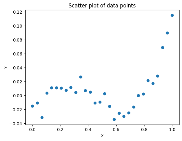
I’m going to generate some data for us to play with. It actually comes from a cubic but lets pretend we don’t know that yet.

data_x = np.linspace(0, 1, 30)
data_y = (data_x-.1)*(data_x-.4)*(data_x-.8) + 0.01 * np.random.randn(30)

Write code below to make a scatter plot with the x data on the x-axis and the y data on the y-axis.

## Write code below. ##

Show code cell content

Hide code cell content

### ANSWER  ###

plt.scatter(data_x, data_y)
plt.xlabel('x')
plt.ylabel('y')
plt.title('Scatter plot of data points');

❓❓❓ Question ❓❓❓: Based on the data_x generated above, build the matrices \(\mathbf{S}\) and \(\mathbf{t}\).

# Your answer here, replace the Nones below

S = None 
t = None 

Show code cell content

Hide code cell content

### ANSWER ###

# Note there are lots of ways to build this matrix
S = np.array([[1, data_x[i]] for i in range(len(data_x))])
t = data_y

# To verify, print the first 10 rows of S
print(S[:10,:])

[[1.         0.        ]
 [1.         0.03448276]
 [1.         0.06896552]
 [1.         0.10344828]
 [1.         0.13793103]
 [1.         0.17241379]
 [1.         0.20689655]
 [1.         0.24137931]
 [1.         0.27586207]
 [1.         0.31034483]]

❓❓❓ Question ❓❓❓: Use your matrices \(\mathbf{S}\) and \(\mathbf{t}\) from above to solve the least squares problem \(\min_{\mathbf{x}\in\mathbb{R}^{n}}\|\mathbf{S}\mathbf{x}-\mathbf{t}\|^2\).

# Your answer here 

Show code cell content

Hide code cell content

### ANSWER ###

# Option 1: Using the normal equations
AtA = S.T @ S
Att = S.T @ t
x_ls = np.linalg.inv(AtA) @ Att
print("Using normal equations, least squares solution:")
print(x_ls)

# Option 2: Using lstsq
x_ls2 = np.linalg.lstsq(S, t)[0]
print("Using lstsq, least squares solution:")
print(x_ls2)

Using normal equations, least squares solution:
[-0.01837331  0.05172523]
Using lstsq, least squares solution:
[-0.01837331  0.05172523]

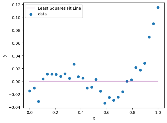
❓❓❓ Question ❓❓❓: Based on the output above, determine \(m\) and \(b\) from the equation \(s_i \approx mt_i + b\) and then plug them in below to plot the line you learned on top of the data.

m = 0 #<- Fix this
b = 0 #<- Fix this too!

plt.plot(data_x, m*data_x + b, color='purple', label='Least Squares Fit Line')
plt.scatter(data_x, data_y, label = 'data')
plt.xlabel('x')
plt.ylabel('y')
plt.legend();

Show code cell content

Hide code cell content

### ANSWER ###
# RANDOM ANSWERS!
# Note this is just to show that different choices give different lines 
# Re-running this cell will give different lines

m = np.random.normal(x_ls[1],.1) #<- 
b = np.random.normal(x_ls[0],.1) #<- 

plt.title('Random Choices of m and b')
plt.plot(data_x, m*data_x + b, color='purple', label='Least Squares Fit Line')
plt.scatter(data_x, data_y, label = 'data')
plt.xlabel('x')
plt.ylabel('y')
plt.legend();

Show code cell content

Hide code cell content

### ANSWER ###

m = x_ls[1] #<- Notice the order, the slope is in the second position in our matrices
b = x_ls[0] #<- 

plt.title('Solution')
plt.plot(data_x, m*data_x + b, color='purple', label='Least Squares Fit Line')
plt.scatter(data_x, data_y, label = 'data')
plt.xlabel('x')
plt.ylabel('y')
plt.legend();

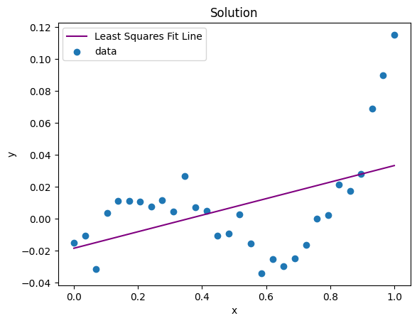
Whelp, that fit isn’t great, but we knew that we didn’t get the data from a line anyway so we didn’t expect a line to do a good job. So, let’s try to fit it with a polynomial instead.

Nonlinear fitting.

Least squares can also be used in polynomial fitting. If we know that the points are approximately related to a polynomial of degree at most \(d\), i.e. for each data point \((s_i,t_i)\),

\[\beta_0 + \beta_1 s_i + \beta_2 s_i^2 + \cdots \beta_d s_i^d \approx t_i\]

then for our input data, we can try to find \(\beta_i\)’s to make

\[\begin{split} \begin{bmatrix} 1 & s_1 & s_1^2 & s_1^3 & \cdots & s_1^d\\ 1 & s_1 & s_1^2 & s_1^3 & \cdots & s_1^d\\ \vdots & \vdots & \vdots & \vdots & & \vdots \\ 1 & s_1 & s_1^2 & s_1^3 & \cdots & s_1^d\\ \end{bmatrix} \begin{bmatrix} \beta_0 \\ \beta_1 \\ \beta_2 \\ \beta_3 \\ \vdots \\ \beta_d \end{bmatrix} \approx \begin{bmatrix} t_0 \\ t_1 \\ t_2 \\ t_3 \\ \vdots \\ t_d \end{bmatrix} \end{split}\]

Notice that the first two columns of \(\mathbf{S}\) matrix are the same as the \(S\) you figured out above. This matrix is called the Vandermonde matrix, so we can just use built in tools to compute it.

S = np.vander(data_x, N=4, increasing=True)
S[:10,:]

array([[1.00000000e+00, 0.00000000e+00, 0.00000000e+00, 0.00000000e+00],
       [1.00000000e+00, 3.44827586e-02, 1.18906064e-03, 4.10020911e-05],
       [1.00000000e+00, 6.89655172e-02, 4.75624257e-03, 3.28016729e-04],
       [1.00000000e+00, 1.03448276e-01, 1.07015458e-02, 1.10705646e-03],
       [1.00000000e+00, 1.37931034e-01, 1.90249703e-02, 2.62413383e-03],
       [1.00000000e+00, 1.72413793e-01, 2.97265161e-02, 5.12526139e-03],
       [1.00000000e+00, 2.06896552e-01, 4.28061831e-02, 8.85645168e-03],
       [1.00000000e+00, 2.41379310e-01, 5.82639715e-02, 1.40637172e-02],
       [1.00000000e+00, 2.75862069e-01, 7.60998811e-02, 2.09930706e-02],
       [1.00000000e+00, 3.10344828e-01, 9.63139120e-02, 2.98905244e-02]])

❓❓❓ Question ❓❓❓:

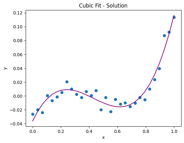
• Use the new, bigger \(\mathbf{S}\) matrix to solve for the coefficients to fit a cubic polynomial, \(t = \beta_0 + \beta_1 s + \beta_2 s^2 + \beta_3s^3\). Hint: You should be able to use exactly the same code as above!

• Then, update the coefficients in the plotting cell below. Does this look like a good fit now?

### Enter your code below.

Show code cell content

Hide code cell content

### ANSWER ###

# Option 1: Using the normal equations
AtA = S.T @ S
Att = S.T @ t
x_ls = np.linalg.inv(AtA) @ Att
print("Using normal equations, least squares solution:")
print(x_ls)

# Option 2: Using lstsq
x_ls2 = np.linalg.lstsq(S, t, rcond=None)[0]
print("Using lstsq, least squares solution:")
print(x_ls2)

Using normal equations, least squares solution:
[-0.02957953  0.44259833 -1.33219335  1.03429624]
Using lstsq, least squares solution:
[-0.02957953  0.44259833 -1.33219335  1.03429624]

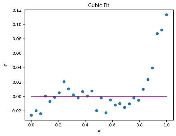
# Fix these with the solution you found to see if the plotted line fits well. 
beta_0 = 0 
beta_1 = 0 
beta_2 = 0
beta_3 = 0

plt.scatter(data_x, data_y, label = 'data')
plt.xlabel('x')
plt.ylabel('y')
plt.plot(data_x, beta_0 + beta_1*data_x + beta_2*data_x**2 + beta_3*data_x**3, color='purple', label='Cubic Least Squares Fit Line');
plt.title('Cubic Fit')

Text(0.5, 1.0, 'Cubic Fit')

Show code cell content

Hide code cell content

### ANSWER ###
beta_0 = x_ls[0]
beta_1 = x_ls[1]
beta_2 = x_ls[2]
beta_3 = x_ls[3]

plt.scatter(data_x, data_y, label = 'data')
plt.xlabel('x')
plt.ylabel('y')
plt.plot(data_x, beta_0 + beta_1*data_x + beta_2*data_x**2 + beta_3*data_x**3, color='purple', label='Cubic Least Squares Fit Line');
plt.title('Cubic Fit - Solution');

Choosing \(d\)

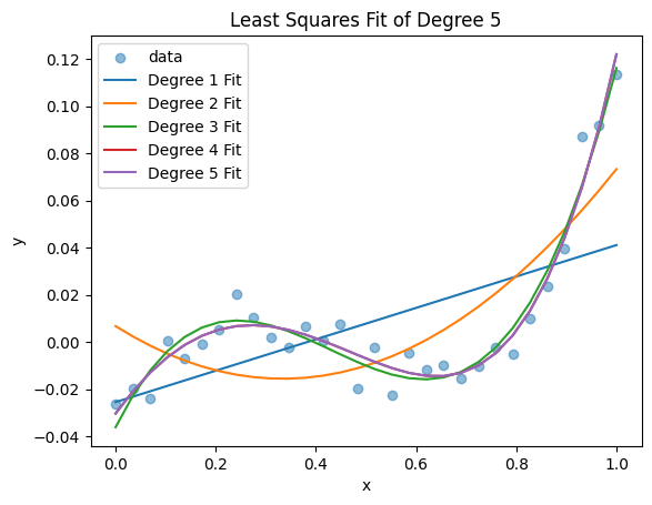
Now, we can try different choices of polynomial degree and see which one fits the best.

❓❓❓ Question ❓❓❓:

• For \(d=1,2,3,4,5\), solve the optimzation problem above and compute the minimum value of the RSS.

• Based on this, which degree polynomial gave the best approximation?

• Plot all of your functions on a scatter plot of the data. Does the visually best fit function match with what you said above?

# Your code here

Show code cell content

Hide code cell content

### ANSWER ###
S = np.vander(data_x, N=5, increasing=True)

RSS = []
    
plt.scatter(data_x, data_y, label='data', alpha=0.5)

for deg in [1, 2, 3, 4, 5]:
    S_deg = S[:, :deg+1]  # Select columns up to degree 'deg'
    x_ls = np.linalg.lstsq(S_deg, t, rcond=None)[0]
    
    # Generate fitted values
    fitted_y = S_deg @ x_ls
    
    # Calculate RSS
    residuals = t - fitted_y
    rss = np.sum(residuals**2)
    RSS.append((deg, rss))
    print(f'Degree {deg} RSS: {rss}')
    
    # Plotting
    plt.plot(data_x, fitted_y, label=f'Degree {deg} Fit')
    
plt.xlabel('x')
plt.ylabel('y')
plt.title(f'Least Squares Fit of Degree {deg}')
plt.legend();

Degree 1 RSS: 0.02136830833131003
Degree 2 RSS: 0.013755204408688746
Degree 3 RSS: 0.001990580465887544
Degree 4 RSS: 0.0017698544636081343
Degree 5 RSS: 0.0017698544636081343

© Copyright 2025, The Department of Computational Mathematics, Science and Engineering at Michigan State University.