
Worksheet Chapter 5, Part 2#
Topics#
This section focuses on Chapter 5.2, 5.3 of Beck
This notebook covers:
Cholesky factorization
Damped Newton’s method
Hybrid gradient-Newton method
%matplotlib inline
import matplotlib.pylab as plt
import numpy as np
Code from Last Time#
Before we get started, I’m going to copy in the code previous classes so that we can use it here.
Gradient Method with Backtracking#
# Backtracking line search function

def step_size_backtrack(f, g, x_k, d_k, s=2, alpha=1/4, beta = 0.5):
    """A function to compute the step size using backtracking line search.
    Args:
        f : The objective function. Note this should be a function of some input vector x.
        g : The gradient of the objective function. Again this should be a function of some input vector x.
        x_k : Current point
        d_k : Current search direction #<-- Note added for this notebook
        s : Initial step size (default is 2)
        alpha : Parameter for backtracking (default is 1/4)
        beta : Step size reduction factor in backtracking (default is 0.5)

    Returns:
        t : The step size found using backtracking line search
    """

    t = s

    fun_val = f(x_k)
    grad_x = g(x_k)

    while fun_val - f(x_k + t * d_k) < alpha*t*grad_x.T @ d_k:
        t = beta * t

    return t

def gradient_method_backtrack(f, g, x0, epsilon, s=2, alpha=1/4, beta=0.5, max_iter = 100):
    """A function to minimize x^t A x + 2 b^t x using the gradient method with backtracking line search.

    Args:
        f : The objective function. Note this should be a function of some input vector x.
        g : The gradient of the objective function. Again this should be a function of some input vector x.
        x0 : Initial guess for the solution
        epsilon : Tolerance for the stopping criterion
        max_iter : Maximum number of iterations to perform (default is 100)
        s : Initial step size for backtracking line search (default is 2)
        alpha : Parameter for backtracking (default is 1/4)
        beta : Step size reduction factor in backtracking (default is 0.5)

    Returns:
        x : The vector of inputs that minimizes the objective function
        fun_val : The value of the objective function at the minimum
        x_all : A list of all iterates generated during the optimization
    """
    # Start with initial guess
    x_k = x0
    f_k = f(x_k)  # Initial function value

    # Store all iterates (the x_k's used)
    x_all = [x0]

    # Keep a counter for how many iterations
    ite = 0
    grad_k = g(x_k)
    while np.linalg.norm(grad_k) > epsilon and ite < max_iter:

        grad_k = g(x_k)
        t_k = step_size_backtrack(f, g, x_k, -grad_k, s, alpha, beta) #<----
        d_k = -grad_k

        # Update x_k to the next x_k (x_{k+1} in the notation above)
        x_k = x_k + t_k * d_k

        # Compute the function value at the new iterate
        f_k = f(x_k)

        # Append the new iterate to the list
        x_all.append(x_k)

        ite = ite + 1
        if (ite%1000==0):
           print("iter_number = %3d norm_grad = %2.6f fun_val = %2.6f" %(ite, np.linalg.norm(grad_k), f_k))
        if ite >= max_iter:
            print("Maximum number of iterations reached.")
            break

    x_soln = x_k
    f_soln = f_k

    return x_soln, f_soln, x_all

#------
# Example usage for last class's function, x^2 + 2y^2
#------

def f(x):
    return x[0]**2 + 2 * x[1]**2

def g(x):
    return np.array([2*x[0], 4*x[1]])

x0 = np.array([1.0, 1.0])
epsilon = 1e-6

x_soln, f_soln, x_all = gradient_method_backtrack(f, g, x0, epsilon, s=2, alpha=1/4, beta=0.5, max_iter = 100)

print("Solution x:", x_soln)
print("Function value at solution:", f_soln)
print(f"Number of iterations: {len(x_all)-1}")
Maximum number of iterations reached.
Solution x: [0. 1.]
Function value at solution: 2.0
Number of iterations: 100
Pure Newton’s Method#
def pure_newton(f, g, h, x0, epsilon=1e-5, max_iter=100):
    """A function to minimize a twice-differentiable function using pure Newton's method.

    Args:
        f : The objective function. Note this should be a function of some input vector x.
        g : The gradient of the objective function. Again this should be a function of some input vector x.
        h : The Hessian of the objective function. This should be a function of some input vector x.
        x0 : Initial guess for the solution
        epsilon : Tolerance for the stopping criterion (default is 1e-5)
        max_iter : Maximum number of iterations to perform (default is 100)

    Returns:
        x : The vector of inputs that minimizes the objective function
        fun_val : The value of the objective function at the minimum
        x_all : A list of all iterates generated during the optimization
    """
    # Start with initial guess
    x_k = x0
    f_k = f(x_k)  # Initial function value

    # Store all iterates (the x_k's used)
    x_all = [x0]

    # Keep a counter for how many iterations
    ite = 0
    grad_k = g(x_k)

    while np.linalg.norm(grad_k) > epsilon and ite < max_iter:
        ite = ite + 1

        # Compute Hessian at current point
        hess_k = h(x_k)

        # Compute Newton direction using matrix operations
        d_k = -np.linalg.inv(hess_k) @ grad_k

        # Update x_k to the next x_k (x_{k+1} in the notation above)
        x_k = x_k + d_k

        # Compute the function value at the new iterate
        f_k = f(x_k)
        grad_k = g(x_k)

        # Append the new iterate to the list
        x_all.append(x_k)

        print("iter_number = %3d \t grad = %2.6f \t fun_val = %2.6f" %(ite, np.linalg.norm(grad_k), f_k))

        if ite >= max_iter:
            print("Maximum number of iterations reached.")
            break

    x_soln = x_k
    f_soln = f_k

    return x_soln, f_soln, x_all

# Test it

x0 = np.array([1, 1])
def f(x):
    return x[0]**2 + 2 * x[1]**2
def g(x):
    return np.array([2*x[0], 4*x[1]])
def h(x):
    return np.array([[2, 0], [0, 4]])


x, fun_val, x_all = pure_newton(f, g, h, x0, epsilon=1e-6, max_iter=100)
print("Solution x:", x)
print("Function value at solution:", fun_val)
print(f"Number of iterations: {len(x_all)-1}")
iter_number =   1 	 grad = 0.000000 	 fun_val = 0.000000
Solution x: [0. 0.]
Function value at solution: 0.0
Number of iterations: 1
Damped Newton’s Method#
Example function#
Consider the optimization problem
whose optimal solution is \((0,0)\).
❓❓❓ Question ❓❓❓:
Write functions f, g, and h which return the function value, gradient, and Hessian (respectively) at the given input point.
# your code here
###ANSWER###
f = lambda x: np.sqrt(1+x[0,0]**2)+np.sqrt(1+x[1,0]**2)
g = lambda x: np.array([[x[0,0]/np.sqrt(1+x[0,0]**2)],[x[1,0]/np.sqrt(1+x[1,0]**2)]])
h = lambda x: np.array([[1/(x[0,0]**2+1)**(3/2),0],[0,1/(x[1,0]**2+1)**(3/2)]])

### Tests
x0 = np.array([[10],[10]])
print(f'f=\n{f(x0)}')
print(f'g=\n{g(x0)}')
print(f'g.shape = {g(x0).shape}')
print(f'h=\n{h(x0)}')
print(f'h.shape = {h(x0).shape}')
f=
20.09975124224178
g=
[[0.99503719]
 [0.99503719]]
g.shape = (2, 1)
h=
[[0.00098519 0.        ]
 [0.         0.00098519]]
h.shape = (2, 2)
❓❓❓ Question ❓❓❓: Try running pure newton method with initial point \((10,10)\) for the problem. What happens?
# Enter code below.
✎ Answer question here.
### ANSWER ###

# Uncomment below to run on the new function, but note this causes a runtime warning because it diverges from the solution.
# x = pure_newton(f,g,h, np.array([[10],[10]]))
❓❓❓ Question ❓❓❓: Try a different initial value (e.g., \((0.5,0.5)\)) for the same example below that leads to a different behavior. What do you observe in this case?
# Enter code below.
### ANSWER ###

x = pure_newton(f,g,h, np.array([[0.5],[0.5]]))

# Yay this one converged! We started closer to the solution, so it worked. The one above diverged because we started too far away from the solution.
iter_number =   1 	 grad = 0.175412 	 fun_val = 2.015564
iter_number =   2 	 grad = 0.002762 	 fun_val = 2.000004
iter_number =   3 	 grad = 0.000000 	 fun_val = 2.000000
✎ Answer question here.
❓❓❓ Question ❓❓❓:
Now, run the gradient_method_backtracking function for the same problem with initial point \((10,10)\) and \((s=1, \alpha=0.5, \beta=0.5, \epsilon=10^{-8})\). How does it converge relative to the pure Newton’s method for the same initial point?
# Write your code below.
✎ Answer question here.
### ANSWER ###

[x, fun_val, x_all]=gradient_method_backtrack(f,g, np.array([[10],[10]]), s =1, alpha=1/2, beta=0.5, epsilon=1e-8)
print(f"x =\n{x}")
print(f"Function value = {fun_val}")
print(f"Number of iterations: {len(x_all)-1}")
# It converges, which is better than the pure Newton's method, which diverged. This is because the backtracking line search helps ensure we don't take steps that are too large, which can cause divergence.
x =
[[0.]
 [0.]]
Function value = 2.0
Number of iterations: 14
The algorithm#
We are now going to implement the Damped Newton’s Method discussed in the videos and in class. This algorithm is sketched as follows.
Initialization: Pick \(\mathbf{x}_0\in\mathbb{R}^n\) arbitrarily, and fix \(\varepsilon >0\) tolerance paramter
General step: For \(k=0,1,2,\dots\),
Compute the Newton direction \(\textbf{d}_k\), which is the solution to the linear system \(\nabla^2 f(\textbf{x}_k)\textbf{d}_k = -\nabla f(\textbf{x}_k)\)
Pick \(t_k\) using constant stepsize, exact line search, or backtracking
Set \(\textbf{x}_{k+1} = \textbf{x}_k+{t_k}\textbf{d}_k\)
If \(\|\nabla f(\textbf{x}_{k+1})\| < \varepsilon\), stop and output \(\textbf{x}_{k+1}\).
❓❓❓ Question ❓❓❓: The following function implements Newton’s method with backtracking line search (damped Newton’s method). You need to complete missing parts of the code.
def newton_backtracking(f, g, h, x0, s=1,alpha=1/2, beta=1/2, epsilon=1e-8, maxiter = 1000):
    """A function to minimize a twice-differentiable function using damped Newton's method with backtracking line search.

    Args:
        f : The objective function. Note this should be a function of some input vector x.
        g : The gradient of the objective function. Again this should be a function of some input vector x.
        h : The Hessian of the objective function. This should be a function of some input vector x.
        x0 : Initial guess for the solution
        s : Initial step size (default is 1)
        alpha : Parameter for backtracking (default is 1/2)
        beta : Step size reduction factor in backtracking (default is 1/2)
        epsilon : Tolerance for the stopping criterion (default is 1e-8)
        maxiter : Maximum number of iterations before stopping

    Returns:
        x : The vector of inputs that minimizes the objective function
        x_all : A list of all iterates generated during the optimization
    """
    x = x0
    x_all = [x0]
    grad = g(x)
    hess = h(x)
    ite = 0
    while (np.linalg.norm(grad) > epsilon) & (ite < maxiter):

        #-----
        # Remove break before working
        break
        #----

        ite = ite + 1

        d =  np.linalg.solve(hess, grad)

        t = s
        while f(x) - f(x - t*d) < alpha * t * d.T@grad:
            t = 0 #<--- Update this line
        x = x #<--- Update this line

        x_all.append(x)
        grad = g(x)
        hess = h(x)
        print("iter_number = %3d fun_val = %2.10f" %(ite, f(x)))
        if ite == maxiter:
            print("did not converge!!!")

    return x, f(x), x_all

x0 = np.array([[10],[10]])
x_soln, f_soln, x_all = newton_backtracking(f,g,h, x0)
print(f"x =\n{x}")
print(f"Minimum f(x) = {f_soln}")
print(f"Number of iterations = {len(x_all)-1}")
x =
[[0.]
 [0.]]
Minimum f(x) = 20.09975124224178
Number of iterations = 0
### ANSWER ###

def newton_backtracking(f, g, h, x0, s=1,alpha=1/2, beta=1/2, epsilon=1e-8, maxiter = 1000):
    """A function to minimize a twice-differentiable function using damped Newton's method with backtracking line search.

    Args:
        f : The objective function. Note this should be a function of some input vector x.
        g : The gradient of the objective function. Again this should be a function of some input vector x.
        h : The Hessian of the objective function. This should be a function of some input vector x.
        x0 : Initial guess for the solution
        s : Initial step size (default is 1)
        alpha : Parameter for backtracking (default is 1/2)
        beta : Step size reduction factor in backtracking (default is 1/2)
        epsilon : Tolerance for the stopping criterion (default is 1e-8)
        maxiter : Maximum number of iterations before stopping

    Returns:
        x : The vector of inputs that minimizes the objective function
        x_all : A list of all iterates generated during the optimization
    """
    x = x0
    x_all = [x0]
    grad = g(x)
    hess = h(x)
    ite = 0
    while (np.linalg.norm(grad) > epsilon) & (ite < maxiter):
        ite = ite + 1

        d =  np.linalg.solve(hess, grad)

        t = s
        while f(x) - f(x - t*d) < alpha * t * d.T@grad:
            t = beta*t #<--- Update this line
        x = x - t*d #<--- Update this line

        x_all.append(x)
        grad = g(x)
        hess = h(x)
        # print("iter_number = %3d fun_val = %2.10f" %(ite, f(x)))
        if ite == maxiter:
            print("did not converge!!!")

    return x, f(x), x_all

x0 = np.array([[10],[10]])
x_soln, f_soln, x_all = newton_backtracking(f,g,h, x0)

print(f"x =\n{x_soln}")
print(f"Minimum f(x) = {f_soln}")
print(f"Number of iterations = {len(x_all)-1}")
x =
[[-1.2409524e-15]
 [-1.2409524e-15]]
Minimum f(x) = 2.0
Number of iterations = 18
❓❓❓ Question ❓❓❓: Run the Newton’s method with backtracking line search for \(x_0 = [10,10]\) and for \([0.5,0.5]\). Does it converge? How do these compare to the pure Newton’s method? To the backtracking method?
x0 = np.array([[10],[10]])
x_soln, f_soln, x_all = newton_backtracking(f,g,h, x0)

print(f"x =\n{x}")
print(f"Minimum f(x) = {f_soln}")
print(f"Number of iterations = {len(x_all)-1}")
x =
[[0.]
 [0.]]
Minimum f(x) = 2.0
Number of iterations = 18
x0 = np.array([[0.5],[0.5]])
x_soln, f_soln, x_all = newton_backtracking(f,g,h, x0)

print(f"x =\n{x}")
print(f"Minimum f(x) = {f_soln}")
print(f"Number of iterations = {len(x_all)-1}")
x =
[[0.]
 [0.]]
Minimum f(x) = 2.0
Number of iterations = 14
✎ Answer question here.
###ANSWER##
# For the x0 = [10,10] case, it converges in 18 iterations while pure Newton's method diverged for this case. However, in both cases it took more iterations in the case of x=[0.5,0.5] for the backtracking line search method than for pure Newton's method, which converged in 3 iterations for that case. This is because the backtracking line search takes smaller steps to ensure convergence, which can lead to more iterations, while pure Newton's method can take larger steps that may converge faster if it doesn't diverge.
The Cholesky Factorization#
The Cholesky decomposition can be used to tackle two issues: validating whether the Hessian matrix is positive definite, and solving the system of equations \(\nabla^2 f(\mathbf{x}_k)\mathbf{d}_k=-\nabla f(\mathbf{x}_k)\).
Given an \(n\times n\) positive definite matrix \(A\), a Cholesky factorization has the form
where \(L\) is a lower triangular \(n\times n\) matrix with a positive diagonal.
In this class you are not required to know how to compute the Cholesky facotorization by hand, but you do need to know how to make Python do it for you using the numpy.linalg.cholesky function
# Uncomment below to get information about the function
# ?np.linalg.cholesky
❓❓❓ Question ❓❓❓: Compute the Cholesky factorization for
and then check that the output satisfies \(A = LL^\top\).
# write your answer here
### ANSWER ###
A1 = np.array([[9, 3, 3], [3, 17, 21], [3, 21, 107]])

L1 = np.linalg.cholesky(A1)

print("Cholesky Factor for 1:\n", L1)

print("\nLL^T = \n", L1 @ L1.T)
Cholesky Factor for 1:
 [[3. 0. 0.]
 [1. 4. 0.]
 [1. 5. 9.]]

LL^T =
 [[  9.   3.   3.]
 [  3.  17.  21.]
 [  3.  21. 107.]]
❓❓❓ Question ❓❓❓: Try to compute the Cholesky factorization for
This should throw an error… what went wrong?
# Your code here
###ANSWER###
A2 = np.array([[2, 4, 7], [4, 6, 7], [7, 7, 4]])

print("Eigenvalues of A2:\n", np.linalg.eigvals(A2))
print("Note that they are not all positive, so A2 is not positive definite.\n")
print("that means we cannot compute the Cholesky factorization of A2.\n")

# Uncomment the code below to see the error message, which will also tell you that the input wasn't positive definite.
# L2 = np.linalg.cholesky(A2)
Eigenvalues of A2:
 [16.24769461 -4.46809185  0.22039724]
Note that they are not all positive, so A2 is not positive definite.

that means we cannot compute the Cholesky factorization of A2.
Hybrid Gradient-Newton Method#
The idea behind the Hybrid Gradient-Newton method is as follows:
When deciding on \(d_k\), we check whether or not the Hessian matrix is positive definite.
If it is positive definite, we use the Newton method.
If it’s not positive definite, we can’t use Newton method. So we fall back to using the gradient method.
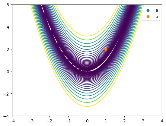
Rosenbrock function (again)#
We are going to test this on the Rosenbrock function
Which is the function we used on the Jupyter notebook for 4-2 as an example for something that converged very slowly when using the gradient method.
Below are the functions to give us the Rosenbrock function (f), it’s gradient (g), and its Hessian (h), as well as a funciton to easily plot the function
f = lambda x: 100*(x[1]-x[0]**2)**2+(1-x[0])**2
g = lambda x: np.array([-400*(x[1]-x[0]**2)*x[0]-2*(1-x[0]), 200*(x[1]-x[0]**2)])
h = lambda x: np.array([[-400*x[1]+1200*x[0]**2+2,-400*x[0]],[-400*x[0],200]])
def plot_rosen(ax = None):
    if ax is None:
        fig, ax = plt.subplots()

    x = np.linspace(-4, 4, 1000)
    y = np.linspace(-4, 6, 1000)
    xmesh, ymesh = np.meshgrid(x,y)

    f = lambda x: 100*(x[1]-x[0]**2)**2+(1-x[0])**2
    fmesh = f(np.array([xmesh, ymesh]))

    plt.contour(xmesh, ymesh, fmesh, np.logspace(0, 3, 30));

    return ax

plot_rosen();
plt.show()

We are going to focus on two specific points while we’re playing around:
For \(a = (1,0)\), the Hessian is positive definite.
For \(b = (1,2)\), the Hessian is indefinite.
a = np.array((1,0))
b = np.array((1,2))

print(f"h(a)=\n{h(a)}")
print(f"eigenvalues of h(a): {np.linalg.eigvals(h(a))}")
print("\n")
print(f"h(b)=\n{h(b)}")
print(f"eigenvalues of h(b): {np.linalg.eigvals(h(b))}")

plot_rosen()
plt.scatter([a[0]], a[1], label = 'a', zorder = 10)
plt.scatter([b[0]], b[1], label = 'b', zorder = 10)
plt.legend()
plt.show()
h(a)=
[[1202 -400]
 [-400  200]]
eigenvalues of h(a): [1342.09359691   59.90640309]


h(b)=
[[ 402 -400]
 [-400  200]]
eigenvalues of h(b): [ 713.55423886 -111.55423886]
Deciding on \(d_k\)#
Assume that \(h_k = h(x_k)\) is the Hessian matrix at step \(k\), and \(g_k = g(x_k)\) is the gradient at step \(k\).
Now we need to write a function that either returns the \(d_k\) that makes \(h_k \cdot d_k = -g_k\) (Newton Method) or returns \(d_k = -g_k\), which is just the negative gradient direction.
First, let’s assume that \(h_k\) is positive definite so that we are going to have to solve for the Newton direction where \(d_k\) solves \(h_k \cdot d_k = -g_k\). We could just use the matrix inverse to solve
however, computing the matrix inverse is computationally expensive and prone to numerical errors. So we’re going to pull a trick with the Cholesky decomposition we just learned to make this work better.
Since \(h_k\) is positive definite by assumption, it has a Cholesky decomposition, specifically there is a matrix \(L\) with
This means our problem above turns into finding \(d_k\) so that
Now let \(u = L^\top d_k\) (we’ll figure out what it is in a minute), so we can solve for \(u\) that makes
Now that we have the \(u\) that makes the above true, we can then solve the equation
for \(d_k\) since \(u\) and \(L\) are now fixed.
❓❓❓ Question ❓❓❓:
We’re going to start using the np.linalg.solve function, where np.linalg.solve(A,b) returns the x so that Ax=b. Information on this function is below.
In the following cell, using the assumption that \(h_k\) is positive definite and testing this at the point \(a = (1,0)\) we checked above, write the code that will compute \(d_k\) for these inputs using the process described above. Check your answer on the figure below, does it look like you’re going in the right direction?
# Uncomment for info on the function
# ?np.linalg.solve
a = np.array((1,0))

g_k = g(a)
h_k = h(a)

L = None #<--- Update this line to compute the Cholesky factor of h_k
u = None #<--- Update this line to solve for u in L u = -g_k
d_k = None #<--- Update this line to solve for d_k in L^T d_k = u

print(d_k)
None
###ANSWER###

a = np.array((1,0))

g_k = g(a)
h_k = h(a)

L = np.linalg.cholesky(h_k)
u = np.linalg.solve(L, -g_k)
d_k = np.linalg.solve(L.T, u)

print(d_k)
[0. 1.]
plot_rosen()
plt.scatter([a[0]], a[1], label = 'a', zorder = 10, color = 'black')
plt.plot([a[0], a[0]+d_k[0]], [a[1], a[1]+d_k[1]], label = 'd_k', zorder = 10, color = 'black')
plt.legend()
plt.show()

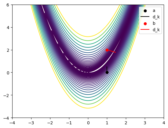
❓❓❓ Question ❓❓❓:
Now we can use this to figure out the direction to used based on \(g_k\) and \(h_k\) for any input case. The issue is that if \(h_k\) is not positive definite, we can’t use Newton’s method. As soon as you try to get its Cholesky decomposition, the code will throw a np.linalg.LinAlgError. We use this in the following skeleton code so that you either try to get Newton’s direction, or you fall back to the negative of the gradient.
Update the code below using the code you wrote above to choose the direction based on the gradient and Hessian inputs at \(x_k\). You can check for reasonableness of the direction using the plot below.
def get_hybrid_d(g_k, h_k):

    try:
        # Use your code from above to get Newton's direction
        L = None
        u = None
        d_k = None
    except np.linalg.LinAlgError:
        # If you get an error from trying to do Cholesky,
        # Use the negative gradient direction instead
        d_k = None

    return d_k
###ANSWER###
def get_hybrid_d(g_k, h_k):

    try:
        # Get Newton's direction
        L = np.linalg.cholesky(h_k)
        u = np.linalg.solve(L, -g_k)
        d_k = np.linalg.solve(L.T, u)
    except np.linalg.LinAlgError:
        # If Cholesky fails (not positive definite),
        # use negative gradient direction
        d_k = -g_k

    return d_k
plot_rosen()

# Figure out the direction for point a and plot
plt.scatter([a[0]], a[1], label = 'a', zorder = 10, color = 'black')
d_k = get_hybrid_d(g(a), h(a))
d_k_scaled = 0.5 * d_k / np.linalg.norm(d_k) # Scale the direction for better visualization
plt.plot([a[0], a[0]+d_k_scaled[0]], [a[1], a[1]+d_k_scaled[1]], label = 'd_k', zorder = 10, color = 'black')

# Figure out the direction for point b and plot
plt.scatter([b[0]], b[1], label = 'b', zorder = 10, color = 'red')
d_k = get_hybrid_d(g(b), h(b))
d_k_scaled = 0.5 * d_k / np.linalg.norm(d_k) # Scale the direction for better visualization
plt.plot([b[0], b[0]+d_k_scaled[0]], [b[1], b[1]+d_k_scaled[1]], label = 'd_k', zorder = 10, color = 'red')


plt.legend()
plt.show()
Hybrid Newton Code#
❓❓❓ Question ❓❓❓: Now we can put this all together. Fill in the missing bits from the code using the functions built earlier in the notebook.
def newton_hybrid(f, g, h, x0, alpha=1/4, beta=0.5, epsilon=1e-6, max_iter=10000):
    """
    Hybrid-Newton method for a twice differentiable function. This method uses Newton's method when the Hessian is positive definite, and falls back to the gradient method otherwise.

    Args:
        f : The objective function
        g : Gradient of the objective function
        h : Hessian of the objective function
        x0 : Initial point
        alpha : Tolerance parameter for the stepsize selection strategy (default: 1/4)
        beta : Proportion in which the stepsize is multiplied at each
        backtracking step, 0 < beta < 1 (default: 0.5)
        epsilon : Tolerance parameter for stopping rule (default: 1e-6)
        max_iter : Maximum number of iterations to perform (default: 10000)

    Returns:
        x : Optimal solution (up to a tolerance)
        fun_val : Optimal function value
        all_x : List of all iterates generated during the optimization
    """

    #--- Remove return before working. This is to keep
    #--- the notebook from throwing errors
    return

    all_x = [x0]
    x_k = x0
    g_k = g(x_k)
    h_k = h(x_k)

    iter_count = 0

    while (np.linalg.norm(g_k) > epsilon) and (iter_count < max_iter):
        iter_count += 1

        # Check positive definiteness and compute Newton direction or gradient
        d_k = None # <-- Use the function you created earlier to pick direction

        # Backtracking line search
        t = None # <-- Use the step_size_backtrack function
                 #     from the top of the notebook to pick t

        # Update x
        x_k = None #<---- Update x_k using what you've figured out above
        all_x.append(x_k)
        print(f'iter= {iter_count:2d} f(x)={f(x_k):10.10f}')

        # Update gradient and Hessian
        g_k = g(x_k)
        h_k = h(x_k)

    if iter_count == max_iter:
        print('did not converge')

    return x_k, f(x_k), all_x
##ANSWER##

def newton_hybrid(f, g, h, x0, alpha=1/4, beta=0.5, epsilon=1e-6, max_iter=10000):
    """
    Hybrid-Newton method for a twice differentiable function. This method uses Newton's method when the Hessian is positive definite, and falls back to the gradient method otherwise.

    Args:
        f : The objective function
        g : Gradient of the objective function
        h : Hessian of the objective function
        x0 : Initial point
        alpha : Tolerance parameter for the stepsize selection strategy (default: 1/4)
        beta : Proportion in which the stepsize is multiplied at each
        backtracking step, 0 < beta < 1 (default: 0.5)
        epsilon : Tolerance parameter for stopping rule (default: 1e-6)
        max_iter : Maximum number of iterations to perform (default: 10000)

    Returns:
        x : Optimal solution (up to a tolerance)
        fun_val : Optimal function value
        all_x : List of all iterates generated during the optimization
    """

    all_x = [x0]
    x_k = x0
    g_k = g(x_k)
    h_k = h(x_k)

    iter_count = 0

    while (np.linalg.norm(g_k) > epsilon) and (iter_count < max_iter):
        iter_count += 1

        # Check positive definiteness and compute Newton direction or gradient
        d_k = get_hybrid_d(g_k, h_k)

        # Backtracking line search
        t = step_size_backtrack(f, g, x_k, d_k, s=1, alpha=alpha, beta=beta)

        # Update x
        x_k = x_k + t*d_k
        all_x.append(x_k)
        print(f'iter= {iter_count:2d} f(x)={f(x_k):10.10f}')

        # Update gradient and Hessian
        g_k = g(x_k)
        h_k = h(x_k)

    if iter_count == max_iter:
        print('did not converge')

    return x_k, f(x_k), all_x
# If your code works above, you should be able to use the code below to converge in about 17 iterations.

f = lambda x: 100*(x[1]-x[0]**2)**2+(1-x[0])**2
g = lambda x: np.array([-400*(x[1]-x[0]**2)*x[0]-2*(1-x[0]), 200*(x[1]-x[0]**2)])
h = lambda x: np.array([[-400*x[1]+1200*x[0]**2+2,-400*x[0]],[-400*x[0],200]])

x, f_opt, x_all_hybrid = newton_hybrid(f, g, h, np.array([2.,5.]))

print(f"x = {x}")
iter=  1 f(x)=67.2297895791
iter=  2 f(x)=1.9074455106
iter=  3 f(x)=1.5505920834
iter=  4 f(x)=1.1673731843
iter=  5 f(x)=0.8352415395
iter=  6 f(x)=0.6118808286
iter=  7 f(x)=0.3889329840
iter=  8 f(x)=0.3863613500
iter=  9 f(x)=0.1303229855
iter= 10 f(x)=0.0901655401
iter= 11 f(x)=0.0316994139
iter= 12 f(x)=0.0296695772
iter= 13 f(x)=0.0013869007
iter= 14 f(x)=0.0001744627
iter= 15 f(x)=0.0000000369
iter= 16 f(x)=0.0000000000
iter= 17 f(x)=0.0000000000
x = [1. 1.]
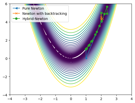
❓❓❓ Question ❓❓❓: Fill in the code to compute the optimum of the Rosenbrock function using pure Newton, and then Newton with backtracking from our function above.
# Uncomment and fix below.

# x, f_opt, x_all_newton = #<--- Update this line to run pure Newton's method without backtracking line search
# print(f"Number of iterations: {len(x_all_newton)-1}")

# x, f_opt, x_all_newton_back = #<--- Update this line to run pure Newton's method with backtracking line search
# print(f"Number of iterations: {len(x_all_newton_back)-1}")
###ANSWER###
x, f_opt, x_all_newton = pure_newton(f,g,h, np.array([2.,5.]))
print(f"Number of iterations: {len(x_all_newton)-1}")

x, f_opt, x_all_newton_back = newton_backtracking(f,g,h, np.array([2.,5.]))
print(f"Number of iterations: {len(x_all_newton_back)-1}")
iter_number =   1 	 grad = 2.030309 	 fun_val = 1.010076
iter_number =   2 	 grad = 449.007817 	 fun_val = 99.989976
iter_number =   3 	 grad = 0.010051 	 fun_val = 0.000025
iter_number =   4 	 grad = 0.011293 	 fun_val = 0.000000
iter_number =   5 	 grad = 0.000000 	 fun_val = 0.000000
Number of iterations: 5
did not converge!!!
Number of iterations: 1000
plot_rosen()

it_array = np.array(x_all_newton)
plt.plot(it_array.T[0],it_array.T[1],'<-', label = 'Pure Newton')

it_array = np.array(x_all_newton_back)
plt.plot(it_array.T[0],it_array.T[1],'x-', label = 'Newton with backtracking')

it_array = np.array(x_all_hybrid)
plt.plot(it_array.T[0],it_array.T[1],'o-', label = 'Hybrid-Newton')
plt.legend()
plt.show()
© Copyright 2025, The Department of Computational Mathematics, Science and Engineering at Michigan State University.