Jupyter Notebook

Jupyter Notebook#

Lecture 25: Random Forests#

In this module we are going to set up random forest models.

# Everyone's favorite standard imports
import numpy as np
import pandas as pd
import matplotlib.pyplot as plt
%matplotlib inline
import time


# ML imports we've used previously
from sklearn.model_selection import train_test_split
from sklearn.metrics import mean_squared_error

Loading the data#

Since we’re doing regression trees, again, we’re going to use the Carseat data where we will predict Sales from the rest of the columns. I’ll do a bit of cleanup for you so we can get to the good stuff.

url = "https://msu-cmse-courses.github.io/CMSE381-S26/_downloads/2cec98f7fc943558992925bc2510bb9d/Carseats.csv"
carseats = pd.read_csv(url).drop('Unnamed: 0', axis=1)
carseats.ShelveLoc = pd.factorize(carseats.ShelveLoc)[0]
carseats.Urban = carseats.Urban.map({'No':0, 'Yes':1})
carseats.US = carseats.US.map({'No':0, 'Yes':1})
carseats.info()

<class 'pandas.core.frame.DataFrame'>
RangeIndex: 400 entries, 0 to 399
Data columns (total 11 columns):
 #   Column       Non-Null Count  Dtype  
---  ------       --------------  -----  
 0   Sales        400 non-null    float64
 1   CompPrice    400 non-null    int64  
 2   Income       400 non-null    int64  
 3   Advertising  400 non-null    int64  
 4   Population   400 non-null    int64  
 5   Price        400 non-null    int64  
 6   ShelveLoc    400 non-null    int64  
 7   Age          400 non-null    int64  
 8   Education    400 non-null    int64  
 9   Urban        400 non-null    int64  
 10  US           400 non-null    int64  
dtypes: float64(1), int64(10)
memory usage: 34.5 KB

X = carseats.drop(['Sales'], axis = 1)
y = carseats.Sales
X.head()

	CompPrice	Income	Advertising	Population	Price	ShelveLoc	Age	Education	Urban	US
0	138	73	11	276	120	0	42	17	1	1
1	111	48	16	260	83	1	65	10	1	1
2	113	35	10	269	80	2	59	12	1	1
3	117	100	4	466	97	2	55	14	1	1
4	141	64	3	340	128	0	38	13	1	0

Bagging#

Last time, we figured out how to use sklearn.tree.DecisionTreeRegressor to build a single tree to do our regression, but we’d like to be able to use ensemble models to create a pile of trees to give a more robust predction.

Let’s try doing this the hard way first. We’re going to set up the bagging on our carseats data. We’ll use \(B=3\) to create our bagged model. So, step one is to generate three bootstrap samples, meaning I generate data sets by sampling \(n=400\) points with replacement.

X1 = carseats.sample(frac = 1, replace = True, random_state = 42)
y1 = X1.Sales
X1 = X1.drop(['Sales'], axis = 1)

X2 = carseats.sample(frac = 1, replace = True, random_state = 43)
y2 = X2.Sales
X2 = X2.drop(['Sales'], axis = 1)

X3 = carseats.sample(frac = 1, replace = True, random_state = 44)
y3 = X3.Sales
X3 = X3.drop(['Sales'], axis = 1)

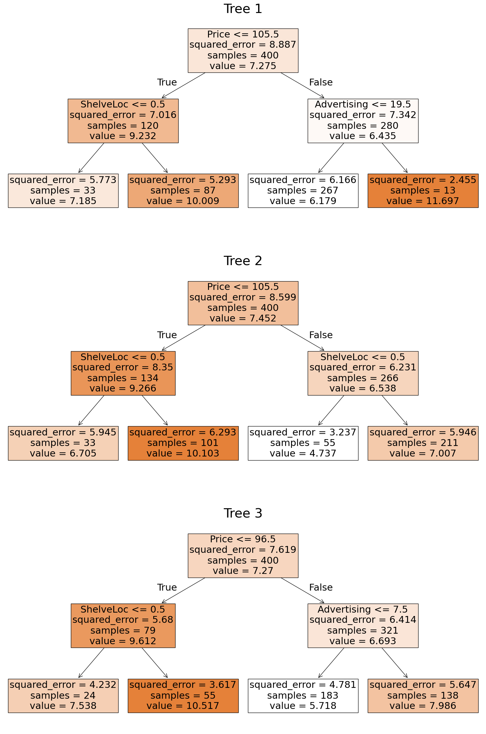
✅ Do this: Fit one regression tree of depth 2 per sampled data we just created. You’ll end up with three regression trees: call them reg_tree1, reg_tree2, and reg_tree3. How similar are the tree structures?

from sklearn import tree
from sklearn.tree import DecisionTreeRegressor

# Your code to generate the three trees here #

# If you named your models reg_tree1, reg_tree2, and reg_tree3 above, 
# this block will plot the three trees
fig, axs = plt.subplots(3,1, figsize = (20,30))

for i, reg_treeX in enumerate([reg_tree1, reg_tree2, reg_tree3]):
    _= tree.plot_tree(reg_treeX, feature_names = X.columns, 
               filled = True, 
              fontsize = 22, 
              ax = axs[i])

    axs[i].set_title(f"Tree {i+1}", fontsize = 30)
plt.show()  

../../../_images/0a37674fa09ed15034a512f4bf8c57bef61f8f00ffd9f6dab885e2d5219ab0df.png

✅ Do this: Predict the Sales value for the first data point in the carseats data set using each of the three trees just generated. What is the average value of the three numbers? This is the bagged prediction for this input data.

X.head().iloc[0,:]

CompPrice      138
Income          73
Advertising     11
Population     276
Price          120
ShelveLoc        0
Age             42
Education       17
Urban            1
US               1
Name: 0, dtype: int64

# Your code to get the bagged prediction for the first here.

Great, you got to here! Hang out for a bit, there’s more lecture before we go on to the next portion.

Random Forests#

Did you really need to do all that bagging by hand? Well, no actually, but this goes under the “eating your vegetables exactly once” part of the lab. Of course, sklearn has built in functions to do bagging for us. In reality, it just has a random forest function, but if we really want to do bagging, we can cheat.

Remember, for random forests, we essentially do bagging but we only allow for a subset of \(m \leq p\) variables to be considered at each splitting step. So if we want bagging, we set the \(m=\)max_features to be the total number of features. That means this next code actually replecates what we just did above with bagging.

from sklearn.ensemble import RandomForestRegressor

# Note we have p=10 input variables
print(X.shape)

(400, 10)

bagged_carseats = RandomForestRegressor(max_features = 10, oob_score = True )
bagged_carseats.fit(X,y)

RandomForestRegressor(max_features=10, oob_score=True)

In a Jupyter environment, please rerun this cell to show the HTML representation or trust the notebook.
On GitHub, the HTML representation is unable to render, please try loading this page with nbviewer.org.

✅ Do this: Build a random forest model instead where the maximum number of features used at each step is \(m = \sqrt {p}\).

# Your code here #

Because we have that oob_score = True set, we get access to the out of bag predictions (i.e., \(\hat y\)) from forest_carseats.oob_prediction_. That is, for each data point, predict its \(\hat y\) by returning the averaged value using only the trees it wasn’t involved in fitting.

##ANSWER##
print(forest_carseats.oob_prediction_.shape)
print(y.shape)
# forest_carseats.oob_prediction_

(400,)
(400,)

✅ Do this: Determine the OOB error on the forest model you built just above using the mean_squared_error command.

Note: The class does also keep track of the oob score as model.oob_score_, however this appears to be reporting \(R^2\) (where close to 1 is better) and I don’t seem to have the ability to change this. See the documentation for further details.

# Your code here

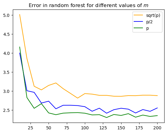
✅ Do this: How does the number of trees used (n_estimators in this code) affect the error? Generate a plot like Fig 8.10 in the book for our carseats data. How many trees should we use?

# Modify the code below to fit a bunch of models and keep track of the MSE.
p = 10

m_list = [int(np.sqrt(p)), int(p/2), int(p)]
print('m_list:', m_list)

n_tree_list = np.arange(10,201,10)

Errors = []
for m in m_list:
    M_error = []
    for i in range(len(n_tree_list)):
        n_trees = n_tree_list[i]
        
        #--------------------------------------------------
        # Add code here to train a random forest model with 
        # max_features = m, n_estimators = n_trees,
        # and the MSE saved as the error below.
        
        error = 0 # <----- your error goes here.
        
        #--------------------------------------------------
        
        M_error.append(error)
    Errors.append(np.array(M_error))

m_list: [3, 5, 10]

# If your code above works, below you'll get a plot of the different choices of m
colors = ['orange','blue','green']
labels = ['sqrt(p)', 'p/2', 'p']

for i in range(3):
    M_error = Errors[i]
    plt.plot(n_tree_list, M_error, label = labels[i], color = colors[i])

plt.legend()
plt.title('Error in random forest for different values of $m$')

plt.show()

../../../_images/24238dc9edba3bc34aeca22ca71e3a68b9d7b6cb02dfcb08b16a6d1138f0828d.png

Congratulations, we’re done!#

Initially created by Dr. Liz Munch, modified by Dr. Lianzhang Bao and Dr. Firas Khasawneh, Michigan State University

This work is licensed under a Creative Commons Attribution-NonCommercial 4.0 International License.

	n_estimators n_estimators: int, default=100 The number of trees in the forest. .. versionchanged:: 0.22 The default value of ``n_estimators`` changed from 10 to 100 in 0.22.	100
	criterion criterion: {"squared_error", "absolute_error", "friedman_mse", "poisson"}, default="squared_error" The function to measure the quality of a split. Supported criteria are "squared_error" for the mean squared error, which is equal to variance reduction as feature selection criterion and minimizes the L2 loss using the mean of each terminal node, "friedman_mse", which uses mean squared error with Friedman's improvement score for potential splits, "absolute_error" for the mean absolute error, which minimizes the L1 loss using the median of each terminal node, and "poisson" which uses reduction in Poisson deviance to find splits. Training using "absolute_error" is significantly slower than when using "squared_error". .. versionadded:: 0.18 Mean Absolute Error (MAE) criterion. .. versionadded:: 1.0 Poisson criterion.	'squared_error'
	max_depth max_depth: int, default=None The maximum depth of the tree. If None, then nodes are expanded until all leaves are pure or until all leaves contain less than min_samples_split samples.	None
	min_samples_split min_samples_split: int or float, default=2 The minimum number of samples required to split an internal node: - If int, then consider `min_samples_split` as the minimum number. - If float, then `min_samples_split` is a fraction and `ceil(min_samples_split * n_samples)` are the minimum number of samples for each split. .. versionchanged:: 0.18 Added float values for fractions.	2
	min_samples_leaf min_samples_leaf: int or float, default=1 The minimum number of samples required to be at a leaf node. A split point at any depth will only be considered if it leaves at least ``min_samples_leaf`` training samples in each of the left and right branches. This may have the effect of smoothing the model, especially in regression. - If int, then consider `min_samples_leaf` as the minimum number. - If float, then `min_samples_leaf` is a fraction and `ceil(min_samples_leaf * n_samples)` are the minimum number of samples for each node. .. versionchanged:: 0.18 Added float values for fractions.	1
	min_weight_fraction_leaf min_weight_fraction_leaf: float, default=0.0 The minimum weighted fraction of the sum total of weights (of all the input samples) required to be at a leaf node. Samples have equal weight when sample_weight is not provided.	0.0
	max_features max_features: {"sqrt", "log2", None}, int or float, default=1.0 The number of features to consider when looking for the best split: - If int, then consider `max_features` features at each split. - If float, then `max_features` is a fraction and `max(1, int(max_features * n_features_in_))` features are considered at each split. - If "sqrt", then `max_features=sqrt(n_features)`. - If "log2", then `max_features=log2(n_features)`. - If None or 1.0, then `max_features=n_features`. .. note:: The default of 1.0 is equivalent to bagged trees and more randomness can be achieved by setting smaller values, e.g. 0.3. .. versionchanged:: 1.1 The default of `max_features` changed from `"auto"` to 1.0. Note: the search for a split does not stop until at least one valid partition of the node samples is found, even if it requires to effectively inspect more than ``max_features`` features.	10
	max_leaf_nodes max_leaf_nodes: int, default=None Grow trees with ``max_leaf_nodes`` in best-first fashion. Best nodes are defined as relative reduction in impurity. If None then unlimited number of leaf nodes.	None
	min_impurity_decrease min_impurity_decrease: float, default=0.0 A node will be split if this split induces a decrease of the impurity greater than or equal to this value. The weighted impurity decrease equation is the following:: N_t / N * (impurity - N_t_R / N_t * right_impurity - N_t_L / N_t * left_impurity) where ``N`` is the total number of samples, ``N_t`` is the number of samples at the current node, ``N_t_L`` is the number of samples in the left child, and ``N_t_R`` is the number of samples in the right child. ``N``, ``N_t``, ``N_t_R`` and ``N_t_L`` all refer to the weighted sum, if ``sample_weight`` is passed. .. versionadded:: 0.19	0.0
	bootstrap bootstrap: bool, default=True Whether bootstrap samples are used when building trees. If False, the whole dataset is used to build each tree.	True
	oob_score oob_score: bool or callable, default=False Whether to use out-of-bag samples to estimate the generalization score. By default, :func:`~sklearn.metrics.r2_score` is used. Provide a callable with signature `metric(y_true, y_pred)` to use a custom metric. Only available if `bootstrap=True`. For an illustration of out-of-bag (OOB) error estimation, see the example :ref:`sphx_glr_auto_examples_ensemble_plot_ensemble_oob.py`.	True
	n_jobs n_jobs: int, default=None The number of jobs to run in parallel. :meth:`fit`, :meth:`predict`, :meth:`decision_path` and :meth:`apply` are all parallelized over the trees. ``None`` means 1 unless in a :obj:`joblib.parallel_backend` context. ``-1`` means using all processors. See :term:`Glossary ` for more details.	None
	random_state random_state: int, RandomState instance or None, default=None Controls both the randomness of the bootstrapping of the samples used when building trees (if ``bootstrap=True``) and the sampling of the features to consider when looking for the best split at each node (if ``max_features < n_features``). See :term:`Glossary ` for details.	None
	verbose verbose: int, default=0 Controls the verbosity when fitting and predicting.	0
	warm_start warm_start: bool, default=False When set to ``True``, reuse the solution of the previous call to fit and add more estimators to the ensemble, otherwise, just fit a whole new forest. See :term:`Glossary ` and :ref:`tree_ensemble_warm_start` for details.	False
	ccp_alpha ccp_alpha: non-negative float, default=0.0 Complexity parameter used for Minimal Cost-Complexity Pruning. The subtree with the largest cost complexity that is smaller than ``ccp_alpha`` will be chosen. By default, no pruning is performed. See :ref:`minimal_cost_complexity_pruning` for details. See :ref:`sphx_glr_auto_examples_tree_plot_cost_complexity_pruning.py` for an example of such pruning. .. versionadded:: 0.22	0.0
	max_samples max_samples: int or float, default=None If bootstrap is True, the number of samples to draw from X to train each base estimator. - If None (default), then draw `X.shape[0]` samples. - If int, then draw `max_samples` samples. - If float, then draw `max(round(n_samples * max_samples), 1)` samples. Thus, `max_samples` should be in the interval `(0.0, 1.0]`. .. versionadded:: 0.22	None
	monotonic_cst monotonic_cst: array-like of int of shape (n_features), default=None Indicates the monotonicity constraint to enforce on each feature. - 1: monotonically increasing - 0: no constraint - -1: monotonically decreasing If monotonic_cst is None, no constraints are applied. Monotonicity constraints are not supported for: - multioutput regressions (i.e. when `n_outputs_ > 1`), - regressions trained on data with missing values. Read more in the :ref:`User Guide `. .. versionadded:: 1.4	None

	CompPrice	Income	Advertising	Population	Price	ShelveLoc	Age	Education	Urban	US
0	138	73	11	276	120	0	42	17	1	1
1	111	48	16	260	83	1	65	10	1	1
2	113	35	10	269	80	2	59	12	1	1
3	117	100	4	466	97	2	55	14	1	1
4	141	64	3	340	128	0	38	13	1	0

	CompPrice	Income	Advertising	Population	Price	ShelveLoc	Age	Education	Urban	US
0	138	73	11	276	120	0	42	17	1	1
1	111	48	16	260	83	1	65	10	1	1
2	113	35	10	269	80	2	59	12	1	1
3	117	100	4	466	97	2	55	14	1	1
4	141	64	3	340	128	0	38	13	1	0