Jupyter - Day 22 - Secion 001

Lec 22 - Step Functions for Classification

Today we will play with the step functions again! But for classification!

# Everyone's favorite standard imports
import numpy as np
import pandas as pd
import matplotlib.pyplot as plt
%matplotlib inline
import time


# ML imports we've used previously
from sklearn.model_selection import train_test_split
from sklearn.metrics import mean_squared_error
from sklearn.linear_model import LinearRegression

import statsmodels.api as sm

Loading in the data

We’re going to use the Wage data used in the book, so note that many of your plots can be checked by looking at figures in the book.

url = "https://msu-cmse-courses.github.io/CMSE381-S26/_downloads/2d664388c56e51af2d83cea1fe3027f4/Wage.csv"
df = pd.read_csv('../../../DataSets/Wage.csv', index_col =0 )
df.head()

	year	age	sex	maritl	race	education	region	jobclass	health	health_ins	logwage	wage
231655	2006	18	1. Male	1. Never Married	1. White	1. < HS Grad	2. Middle Atlantic	1. Industrial	1. <=Good	2. No	4.318063	75.043154
86582	2004	24	1. Male	1. Never Married	1. White	4. College Grad	2. Middle Atlantic	2. Information	2. >=Very Good	2. No	4.255273	70.476020
161300	2003	45	1. Male	2. Married	1. White	3. Some College	2. Middle Atlantic	1. Industrial	1. <=Good	1. Yes	4.875061	130.982177
155159	2003	43	1. Male	2. Married	3. Asian	4. College Grad	2. Middle Atlantic	2. Information	2. >=Very Good	1. Yes	5.041393	154.685293
11443	2005	50	1. Male	4. Divorced	1. White	2. HS Grad	2. Middle Atlantic	2. Information	1. <=Good	1. Yes	4.318063	75.043154

df.info()

<class 'pandas.core.frame.DataFrame'>
Index: 3000 entries, 231655 to 453557
Data columns (total 12 columns):
 #   Column      Non-Null Count  Dtype  
---  ------      --------------  -----  
 0   year        3000 non-null   int64  
 1   age         3000 non-null   int64  
 2   sex         3000 non-null   object 
 3   maritl      3000 non-null   object 
 4   race        3000 non-null   object 
 5   education   3000 non-null   object 
 6   region      3000 non-null   object 
 7   jobclass    3000 non-null   object 
 8   health      3000 non-null   object 
 9   health_ins  3000 non-null   object 
 10  logwage     3000 non-null   float64
 11  wage        3000 non-null   float64
dtypes: float64(2), int64(2), object(8)
memory usage: 304.7+ KB

df.describe()

	year	age	logwage	wage
count	3000.000000	3000.000000	3000.000000	3000.000000
mean	2005.791000	42.414667	4.653905	111.703608
std	2.026167	11.542406	0.351753	41.728595
min	2003.000000	18.000000	3.000000	20.085537
25%	2004.000000	33.750000	4.447158	85.383940
50%	2006.000000	42.000000	4.653213	104.921507
75%	2008.000000	51.000000	4.857332	128.680488
max	2009.000000	80.000000	5.763128	318.342430

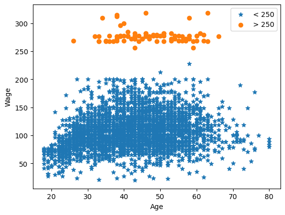
Here’s the plot we used multiple times in class to look at a single variable: age vs wage

plt.scatter(df.age[df.wage <=250], df.wage[df.wage<=250],marker = '*', label = '< 250')
plt.scatter(df.age[df.wage >250], df.wage[df.wage>250], label = '> 250')
plt.legend()

plt.xlabel('Age')
plt.ylabel('Wage')
plt.show()

Classification version of step functions

Now we can try out the classification version of the problem. Let’s build the classifier that predicts whether a person of a given age will make more than $250,000. You already made the matrix of step function features, so we just have to hand it to LogisticRegression to do its thing.

✅ Do this: You will need to first create the dummy variables that represent the step functions. You will need to use pd.cut and pd.get_dummies, or you can copy the relevant code from Day 21’s notebook!

# put your code here

✅ Do this: Pass the dummy variables to a logistic regression model and use it to predict the probability of wage being greater than 250. What is the equation for your learned model? Be specific in terms of the \(C_i\) functions you learned earlier. Complete the code below.

from sklearn.linear_model import LogisticRegression
y = np.array(df.wage>250) #<--- this makes sure I 
                          #     just have true/false input
                          #     so that we're doing classification

# put your code below to fit a logistic regression model #

If all goes well, you should be able to run the below code and plat the prediction.

# Build the same step features for the x-values we want to draw
t_age = pd.Series(np.linspace(20,80,100))
t_df_cut = pd.cut(t_age, bins, right = False) #<-- the `bins`` here is from the initial cut
t_dummies = pd.get_dummies(t_df_cut)
t_step = t_dummies.apply(lambda x: x * 1)

# Predict on these to get the line we can draw
f = clf.predict_proba(t_step)

---------------------------------------------------------------------------
NameError                                 Traceback (most recent call last)
Cell In[8], line 3
      1 # Build the same step features for the x-values we want to draw
      2 t_age = pd.Series(np.linspace(20,80,100))
----> 3 t_df_cut = pd.cut(t_age, bins, right = False) #<-- the `bins`` here is from the initial cut
      4 t_dummies = pd.get_dummies(t_df_cut)
      5 t_step = t_dummies.apply(lambda x: x * 1)

NameError: name 'bins' is not defined

below = df.age[df.wage <=250]
above = df.age[df.wage >250]

# Comment this out to see the function better
# plt.scatter(above,np.ones(above.shape[0]),marker = '|', color = 'orange')
# plt.scatter(below,np.zeros(below.shape[0]),marker = '|', color = 'blue')

plt.xlabel('Age')
plt.ylabel('P[Wage >= 250]')
plt.plot(t_age,f[:,1])
plt.show()

---------------------------------------------------------------------------
NameError                                 Traceback (most recent call last)
Cell In[9], line 10
      8 plt.xlabel('Age')
      9 plt.ylabel('P[Wage >= 250]')
---> 10 plt.plot(t_age,f[:,1])
     11 plt.show()

NameError: name 'f' is not defined

---

Congratulations, we’re done!

Initially created by Dr. Liz Munch, modified by Dr. Lianzhang Bao and Dr. Firas Khasawneh, Michigan State University

This work is licensed under a Creative Commons Attribution-NonCommercial 4.0 International License.