Jupyter - Lecture 7

Even More Linear Regression

In the last few lectures, we have focused on linear regression, that is, fitting models of the form

\[ Y = \beta_0 + \beta_1 X_1 + \beta_2 X_2 + \cdots + \beta_pX_p + \varepsilon \]

In this lab, we will continue to use two different tools for linear regression.

• Scikit learn is arguably the most used tool for machine learning in python

• Statsmodels provides many of the statisitcial tests we’ve been learning in class

This lab will cover two ideas:

• Categorical variables and how to represent them as dummy variables.

• How to build interaction terms and pass them into your favorite model.

# As always, we start with our favorite standard imports. 

import numpy as np
import pandas as pd
import matplotlib.pyplot as plt 
%matplotlib inline
import seaborn as sns
import statsmodels.formula.api as smf

More questions to ask of your model (Continued from last time)

Q3: How well does the model fit?

This section talks about interpretation of \(R^2\) and RSE, but is on slides only.

Q4: Making predictions

url = "https://msu-cmse-courses.github.io/CMSE381-S26/_downloads/27085b33898cca7fb57dc6897c2deccd/Advertising.csv"
advertising_df = pd.read_csv(url, index_col = 0)
# I need to sort the rows by TV to make plotting work better later 
advertising_df= advertising_df.sort_values(by=['TV'])
advertising_df.head()

	TV	Radio	Newspaper	Sales
131	0.7	39.6	8.7	1.6
156	4.1	11.6	5.7	3.2
79	5.4	29.9	9.4	5.3
57	7.3	28.1	41.4	5.5
127	7.8	38.9	50.6	6.6

# I want to just learn Sales using TV
est = smf.ols('Sales ~ TV', advertising_df).fit()
est.params

Intercept    7.032594
TV           0.047537
dtype: float64

# Here is a table giving us the CI and PI information 
alpha = 0.1
# alpha = 0.05
# alpha = 0.01
# alpha = 0.001
advert_summary = est.get_prediction(advertising_df).summary_frame(alpha=alpha)
advert_summary.head()

	mean	mean_se	mean_ci_lower	mean_ci_upper	obs_ci_lower	obs_ci_upper
0	7.065869	0.456216	6.311932	7.819806	1.628140	12.503598
1	7.227494	0.448345	6.486566	7.968422	1.791553	12.663435
2	7.289291	0.445348	6.553316	8.025267	1.854023	12.724559
3	7.379611	0.440981	6.650852	8.108370	1.945316	12.813907
4	7.403379	0.439835	6.676515	8.130244	1.969338	12.837421

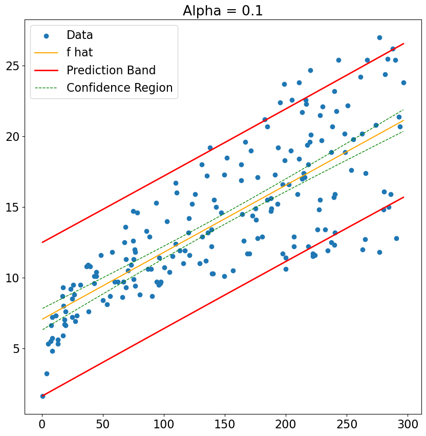
# And here is some code that will draw these beasts for us....
plt.rcParams['figure.figsize'] = [10, 10]
plt.rcParams['font.size'] = 16


x = advertising_df['TV']
y = advertising_df['Sales']


# Plot the original data 
plt.scatter(x,y, label = 'Data')

# Plot the fitted values, AKA f_hat
# you can get this in two different places, same answer
# plt.plot(x,advert_summary['mean'], color = 'orange', label = 'f hat')
plt.plot(x,est.fittedvalues, color = 'orange', label = 'f hat')



plt.plot(x,advert_summary['obs_ci_lower'], 'r', lw=2, 
         label = r'Prediction Band')
plt.plot(x,advert_summary['obs_ci_upper'], 'r', lw=2)

plt.plot(x, advert_summary['mean_ci_lower'],'g--', lw=1, 
         label = r'Confidence Region')
plt.plot(x, advert_summary['mean_ci_upper'], 'g--', lw=1)

plt.title('Alpha = '+ str(alpha))



plt.legend()

<matplotlib.legend.Legend at 0x15b45b510>

Playing with multi-level variables

The wrong way

Ok, we’re going to do this incorrectly to start. You pull in the Auto data set. You were so proud of yourself for remembering to fix the problems with the horsepower column that you conveniently forgot that the column with information about country of origin (origin) has a bunch of integers in it, representing:

• 1: American

• 2: European

• 3: Japanese.

url = "https://msu-cmse-courses.github.io/CMSE381-S26/_downloads/d75c3811a83a66f8c261e5b599ef9e44/Auto.csv"
Auto_df = pd.read_csv(url)
Auto_df = Auto_df.replace('?', np.nan)
Auto_df = Auto_df.dropna()
Auto_df.horsepower = Auto_df.horsepower.astype('int')


Auto_df.columns

Index(['mpg', 'cylinders', 'displacement', 'horsepower', 'weight',
       'acceleration', 'year', 'origin', 'name'],
      dtype='object')

You then go on your merry way building the model $\( \texttt{mpg} = \beta_0 + \beta_1 \cdot \texttt{origin}. \)$

from sklearn.linear_model import LinearRegression

X = Auto_df.origin.values
X = X.reshape(-1, 1)
y = Auto_df.mpg.values

regr = LinearRegression()

regr.fit(X,y)

print('beta_1 = ', regr.coef_[0])
print('beta_0 = ', regr.intercept_)

beta_1 =  5.476547480191433
beta_0 =  14.811973615412484

✅ Q: What does your model predict for each of the three types of cars?

# Your code here

✅ Q: Is it possible for your model to predict that both American and Japanese cars have mpg below European cars?

Your answer here.

The right way

Ok, so you figure out your problem and decide to load in your data and fix the origin column to have names as entries.

convertOrigin= {1: 'American', 2:'European', 3:'Japanese'}

# This command swaps out each number n for convertOrigin[n], making it one of
# the three strings instead of an integer now.
Auto_df.origin = Auto_df.origin.apply(lambda n: convertOrigin[n])
Auto_df

	mpg	cylinders	displacement	horsepower	weight	acceleration	year	origin	name
0	18.0	8	307.0	130	3504	12.0	70	American	chevrolet chevelle malibu
1	15.0	8	350.0	165	3693	11.5	70	American	buick skylark 320
2	18.0	8	318.0	150	3436	11.0	70	American	plymouth satellite
3	16.0	8	304.0	150	3433	12.0	70	American	amc rebel sst
4	17.0	8	302.0	140	3449	10.5	70	American	ford torino
...	...	...	...	...	...	...	...	...	...
392	27.0	4	140.0	86	2790	15.6	82	American	ford mustang gl
393	44.0	4	97.0	52	2130	24.6	82	European	vw pickup
394	32.0	4	135.0	84	2295	11.6	82	American	dodge rampage
395	28.0	4	120.0	79	2625	18.6	82	American	ford ranger
396	31.0	4	119.0	82	2720	19.4	82	American	chevy s-10

392 rows × 9 columns

Below is a quick code that automatically generates our dummy variables. Yay for not having to code that mess ourselves!

origin_dummies_df = pd.get_dummies(Auto_df.origin, prefix='origin')
origin_dummies_df

	origin_American	origin_European	origin_Japanese
0	True	False	False
1	True	False	False
2	True	False	False
3	True	False	False
4	True	False	False
...	...	...	...
392	True	False	False
393	False	True	False
394	True	False	False
395	True	False	False
396	True	False	False

392 rows × 3 columns

✅ Q: What is the interpretation of each column in the origin_dummies_df data frame?

Your answer here

I pass these new dummy variables into my scikit-learn linear regression model and get the following coefficients

X = origin_dummies_df.values
y = Auto_df.mpg

regr = LinearRegression()

regr.fit(X,y)

print('Coefs = ', regr.coef_)
print('Intercept = ', regr.intercept_)

Coefs =  [-1.99394386e+13 -1.99394386e+13 -1.99394386e+13]
Intercept =  19939438589658.2

✅ Q: Now what does your model predict for each of the three types of cars?

# Your code here

Ooops

✅ Q: Aw man, I didn’t quite do what we said for the dummy variables in class. We talked about having only two dummy variables for a three level variable. Copy my code below here and fix it to have two variables instead of three.

• Are your coefficients different now?

• Are your predictions for each of the three origins different now?

• Does it matter which two levels you used for your dummy variables?

# Your code here

##YOUR ANSWER HERE###

##ANSWER## Coefficients are different (in particular, there’s a different number of them) but the prediction ends up the same…..

Another right way

Ok, fine, I’ll cave, I made you do it the hard way but you got to see how the innards worked, so maybe it’s not all bad ;)

First off, we can force sklearn to drop the first variable, so you don’t have to do it manually every time. But you do need to know how to interpret the outputs!

# Even easier right way.... Note the only difference is the drop_first=True
origin_dummies_df = pd.get_dummies(Auto_df.origin, prefix='origin',drop_first=True)
print(origin_dummies_df.head())

y = Auto_df.mpg
regr = LinearRegression()
regr.fit(X,y)

   origin_European  origin_Japanese
0            False            False
1            False            False
2            False            False
3            False            False
4            False            False

LinearRegression()

In a Jupyter environment, please rerun this cell to show the HTML representation or trust the notebook.
On GitHub, the HTML representation is unable to render, please try loading this page with nbviewer.org.

In statsmodels, it can automatically split up the categorical variables in a data frame, so it does the hard work for you. Note that here I’m plugging in the original Auto_df data frame, no processing of the categorical variables on my end at all.

est = smf.ols('mpg ~ origin', Auto_df).fit()
est.summary().tables[1]

	coef	std err	t	P>|t|	[0.025	0.975]
Intercept	20.0335	0.409	49.025	0.000	19.230	20.837
origin[T.European]	7.5695	0.877	8.634	0.000	5.846	9.293
origin[T.Japanese]	10.4172	0.828	12.588	0.000	8.790	12.044

✅ Q: What is the model learned from the above printout? Be specific in terms of your dummy variables.

##Your code or answer here###

---

Congratulations, we’re done!

Initially created by Dr. Liz Munch, modified by Dr.Lianzhang Bao and Dr. Firas Khasawneh, Michigan State University
This work is licensed under a Creative Commons Attribution-NonCommercial 4.0 International License.