Jupyter Day 9 - Section 001#
Lec 9 - Intro to Classification#
# Standard imports
import numpy as np
import matplotlib.pyplot as plt
import pandas as pd
%matplotlib inline
import seaborn as sns
Reading in the chicken or egg data#
In this lab, we are going to try out the KNN classification described in class. First, we’re going to load up our data. This data is 100% made up by Dr. Munch and the code can generate it can be found on the DataSets page. Based on two inputs \(x_1\) and \(x_2\), we get to predict whether we have a chicken or an egg.
Go get the data from the class website then run the following.
url = "https://msu-cmse-courses.github.io/CMSE381-S26/_downloads/bfae9d1905fec60d2deb1e6affcecf8a/ChickenEgg.csv"
Chick_df = pd.read_csv('../../../DataSets/ChickenEgg.csv')
Chick_df.head(10)
| x1 | x2 | Label | |
|---|---|---|---|
| 0 | -3.156478 | -1.110356 | chicken |
| 1 | -3.547711 | 0.438432 | chicken |
| 2 | -6.243875 | 5.288547 | chicken |
| 3 | -5.398701 | 4.044941 | chicken |
| 4 | 3.556318 | 4.750270 | chicken |
| 5 | 3.208898 | -1.319343 | chicken |
| 6 | 6.486065 | -3.953278 | egg |
| 7 | -1.126397 | 3.032450 | chicken |
| 8 | 1.820567 | -6.872025 | egg |
| 9 | -2.601184 | 5.737621 | chicken |
The first step is always to do some data exploration.
✅ Do this: Draw a scatter plot of your data with the relevant labels.
Hint: There are many ways to do this, but sns.scatterplot often works the fastest, and if you set hue and/or style to the Label column, you should get the labels drawn as color and/or symbol.
# Your code here
✅ Do this: Based on your scatter plot, what you expect a KNN classifer with \(k=1\) to predict for a data point at \((-4,4)\)? What about at \((6,0)\)?
Your answer here
KNN with sklearn#
Ok, but let’s be honest, no one is going to do this by hand everytime. Let’s make sklearn do it for us!
from sklearn.neighbors import KNeighborsClassifier
First, we’re going to split our data into two pieces. The \(X\) input variables, and the \(Y\) output variable.
X = Chick_df.drop('Label', axis =1)
y = Chick_df['Label']
X.head()
| x1 | x2 | |
|---|---|---|
| 0 | -3.156478 | -1.110356 |
| 1 | -3.547711 | 0.438432 |
| 2 | -6.243875 | 5.288547 |
| 3 | -5.398701 | 4.044941 |
| 4 | 3.556318 | 4.750270 |
y.head(10)
0    chicken
1    chicken
2    chicken
3    chicken
4    chicken
5    chicken
6        egg
7    chicken
8        egg
9    chicken
Name: Label, dtype: object
Then the following code trains our classifier.
knn = KNeighborsClassifier(n_neighbors=1)
knn.fit(X,y)
KNeighborsClassifier(n_neighbors=1)In a Jupyter environment, please rerun this cell to show the HTML representation or trust the notebook.
On GitHub, the HTML representation is unable to render, please try loading this page with nbviewer.org.
KNeighborsClassifier(n_neighbors=1)
…and this command provides a prediction for an input of \((-2,3)\) input.
knn.predict(pd.DataFrame([[-2, 3]], columns=X.columns))
array(['chicken'], dtype=object)
✅ Do this: What does your classifier predict for \((-4,4)\)? What about at \((6,0)\)? Are these the same that you guessed above?
# Your code here
This predict function is pretty powerful. If I want to get all predictions for all of my inputs, I can just pass my \(X\) dataframe.
knn.predict(X)
array(['chicken', 'chicken', 'chicken', 'chicken', 'chicken', 'chicken',
       'egg', 'chicken', 'egg', 'chicken', 'egg', 'egg', 'chicken', 'egg',
       'egg', 'chicken', 'chicken', 'chicken', 'egg', 'egg', 'egg',
       'chicken', 'chicken', 'egg', 'egg', 'chicken', 'egg', 'chicken',
       'chicken', 'chicken', 'chicken', 'chicken', 'egg', 'chicken',
       'chicken', 'egg', 'chicken', 'chicken', 'egg', 'chicken', 'egg',
       'chicken', 'chicken', 'chicken', 'egg', 'egg', 'egg', 'egg',
       'chicken', 'chicken', 'egg', 'chicken', 'chicken', 'egg',
       'chicken', 'egg', 'egg', 'egg', 'chicken', 'chicken', 'chicken',
       'chicken', 'egg', 'chicken', 'egg', 'chicken', 'chicken',
       'chicken', 'egg', 'chicken', 'egg', 'chicken', 'egg', 'chicken',
       'egg', 'egg', 'chicken', 'egg', 'chicken', 'chicken', 'egg',
       'chicken', 'egg', 'egg', 'egg', 'chicken', 'chicken', 'egg', 'egg',
       'chicken'], dtype=object)
Remember what all the actual labels were?
np.array(y)
array(['chicken', 'chicken', 'chicken', 'chicken', 'chicken', 'chicken',
       'egg', 'chicken', 'egg', 'chicken', 'egg', 'egg', 'chicken', 'egg',
       'egg', 'chicken', 'chicken', 'chicken', 'egg', 'egg', 'egg',
       'chicken', 'chicken', 'egg', 'egg', 'chicken', 'egg', 'chicken',
       'chicken', 'chicken', 'chicken', 'chicken', 'egg', 'chicken',
       'chicken', 'egg', 'chicken', 'chicken', 'egg', 'chicken', 'egg',
       'chicken', 'chicken', 'chicken', 'egg', 'egg', 'egg', 'egg',
       'chicken', 'chicken', 'egg', 'chicken', 'chicken', 'egg',
       'chicken', 'egg', 'egg', 'egg', 'chicken', 'chicken', 'chicken',
       'chicken', 'egg', 'chicken', 'egg', 'chicken', 'chicken',
       'chicken', 'egg', 'chicken', 'egg', 'chicken', 'egg', 'chicken',
       'egg', 'egg', 'chicken', 'egg', 'chicken', 'chicken', 'egg',
       'chicken', 'egg', 'egg', 'egg', 'chicken', 'chicken', 'egg', 'egg',
       'chicken'], dtype=object)
Now, I could sit here and go through one by one to see if they have the same predicted value as the label to decide on my accuracy. But, as usual, sklearn comes to the rescue.
from sklearn.metrics import accuracy_score

accuracy_score(knn.predict(X),y)
1.0
Train test splits#
Ok, so you got 100% accuracy! You’re done, right????
Wrong!
We know better than to report our training accuracy as our actual accuracy! So, let’s set up some basic train/test splits!
from sklearn.model_selection import train_test_split
X_train, X_test, y_train, y_test = train_test_split(X, y, test_size=0.1)
In this case, the X_train data frame has the inputs we’ll use for training…
print(X_train.shape)
X_train.head()
(81, 2)
| x1 | x2 | |
|---|---|---|
| 1 | -3.547711 | 0.438432 |
| 30 | -1.463331 | 6.017793 |
| 55 | -4.015561 | -5.655263 |
| 16 | -4.958622 | 5.982941 |
| 71 | 0.533914 | 5.991084 |
…, and the y_train has the outputs for those same data points.
print(y_train.shape)
y_train.head()
(81,)
1     chicken
30    chicken
55        egg
16    chicken
71    chicken
Name: Label, dtype: object
The X_test data frame has the rest of the inputs which we’ll use for testing, and the y_test has the outputs for those same data points. We don’t get to touch these until after the training is all done! Otherwise we are data-snooping!
print(X_test.shape)
X_test.head(10)
(9, 2)
| x1 | x2 | |
|---|---|---|
| 83 | -5.373723 | -4.728891 |
| 65 | -5.986941 | -1.924147 |
| 80 | -3.692703 | -2.986763 |
| 46 | 1.747229 | -2.692229 |
| 52 | -3.667503 | 5.153813 |
| 82 | -2.186845 | -3.457615 |
| 8 | 1.820567 | -6.872025 |
| 5 | 3.208898 | -1.319343 |
| 69 | -2.976418 | 3.921586 |
print(y_test.shape)
y_test.head(10)
(9,)
83        egg
65    chicken
80        egg
46        egg
52    chicken
82        egg
8         egg
5     chicken
69    chicken
Name: Label, dtype: object
✅ Do this: Build a KNN classifier using \(k=3\) neighbors, and train it on your X_train and y_train data. Call it knn like before.
# Your KNN classifier code here
✅ Do this: Based on the KNN classifier above.
What is your training accuracy?
What is your testing accuracy?
##YOUR ANSWER##
#Training Accuracy


# Testing accuracy
I want to show you one more nice command in here. Remember that KNNs work by returning the label of the most frequently seen label among the \(k\) numbers, but that doesn’t mean every neighbor had that label.
The predict_proba function will tell you the percentage of each that was seen.
knn.predict_proba(X_test)
array([[0.        , 1.        ],
       [1.        , 0.        ],
       [0.33333333, 0.66666667],
       [0.33333333, 0.66666667],
       [1.        , 0.        ],
       [0.        , 1.        ],
       [0.        , 1.        ],
       [0.33333333, 0.66666667],
       [1.        , 0.        ]])
Bayes classifier#
Now, because I generated our data so I know the real Bayes decision boundary, we can take a look at how our results match up with the Bayes classifier.
First, I am going to set up some code that will figure out what your model, named knn above hopfully, will predict for a grid of numbers covering our \([-7,7] \times [-7,7]\) box.
# Run this cell, we just need to generate some inputs
# to be able to draw figures in a moment.
t = np.linspace(-7,7,28)
X_mesh,Y_mesh = np.meshgrid(t,t)
X_mesh_flat = X_mesh.flatten()
Y_mesh_flat = Y_mesh.flatten()

# The test_all_df is a dataframe with all the possible inputs of x1 and x2, so if we predict on all of them we can see the decision boundary.
test_all_df = pd.DataFrame({'x1':X_mesh_flat,'x2':Y_mesh_flat})
pred_all = knn.predict(test_all_df)
def to_int(chickegg):
    if chickegg == 'egg':
        return -1
    else:
        return 1

pred_all = np.array([to_int(x) for x in pred_all])
pred_all.shape
pred_all = pred_all.reshape([28,28])
Then this will plot these predictions on our 2D plane.
plt.pcolor(X_mesh,Y_mesh,pred_all)

cbar = plt.colorbar(ticks=[-1, 1])
cbar.ax.set_yticklabels(['egg','chicken'])

# Just for comparison, I can also plot my original data points on top. Uncomment the line below to see that.
# sns.scatterplot(data = Chick_df, x = 'x1', y = 'x2', style = 'Label').set(title = 'Chicken or Egg?')
[Text(1, -1, 'egg'), Text(1, 1, 'chicken')]
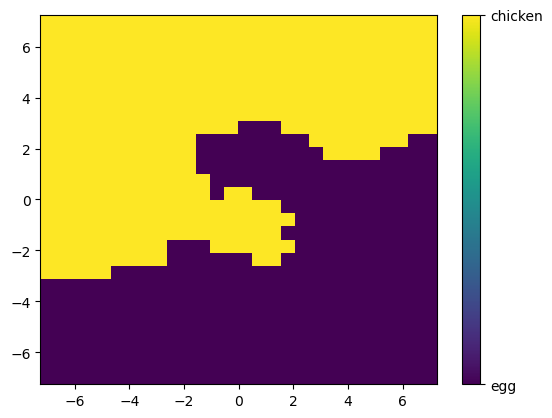
✅ Q: Using this plot, what is your model going to predict for a data point at \((-4,6)\)?
Your answer here
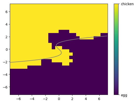
Note that since I generated this data, I know where the line was between the two regions used to generate it. In my case, I happened to use the function
and labeled a new data point based on whether \(f(x_1,x_2) + \varepsilon\) was positive or negative.
Below, you can see \(f(x_1,x_2)\) (in this case, the Bayes classifier) drawn on top of your model’s predictions. How similar did your KNN get?
✅ Q: Where are the regions that your model predicts something different than the Bayes classifier?
# This command tries to draw a line between the two regions
plt.pcolor(X_mesh,Y_mesh,pred_all)

cbar = plt.colorbar(ticks=[-1, 1])
cbar.ax.set_yticklabels(['egg','chicken'])

# This draws the line I used to generate the data
ty = np.linspace(-2.1,2.1,100)
tx = ty**3 - ty
plt.plot(tx,ty, color = 'grey')

# Again, you can uncomment the line below to the original data overlaid.
# sns.scatterplot(data = Chick_df, x = 'x1', y = 'x2', style = 'Label').set(title = 'Chicken or Egg?')
[<matplotlib.lines.Line2D at 0x16853efd0>]
###YOUR ANSWER HERE###
Messing with \(k\)#
Finally, we’re going to generate plots like Fig 2.17 in the book, where we look at the training and testing errors vs the flexibility (in this case, \(1/k\)) of the model used.
# Our choices of $K$
# Note that the graph will use $1/k$ for flexibility
Kinv = np.array([0.04, 0.05,0.2,0.5,1])
Ks = 1/Kinv
Ks = Ks.astype(int)
print(Ks)

Accuracies = []
TrainAccuracies = []


# I'm going to run this model for all my choices of k
for k in Ks:
    thisruntest = []
    thisruntrain = []

    # For each choice of k, i'll do this 10 times and average
    for runNum in range(50):
        X_train, X_test, y_train, y_test = train_test_split(X, y, test_size=0.3)
        knn = KNeighborsClassifier(n_neighbors=k)
        knn.fit(X_train,y_train)

        # Figure out my training error rate
        acctrain = accuracy_score(knn.predict(X_train),y_train)
        thisruntrain.append(1-acctrain)

        # Figure out my testing error rate
        acctest = accuracy_score(knn.predict(X_test),y_test)
        thisruntest.append(1-acctest)

    # Keep the average over the 10 runs
    TrainAccuracies.append(np.average(thisruntrain))
    Accuracies.append(np.average(thisruntest))


# Plot train and test with x-axis on a log scale
plt.semilogx(1/Ks,Accuracies, label = 'Test', marker = 'x')
plt.semilogx(1/Ks,TrainAccuracies, label = 'Train', marker = 'o')
plt.xlabel('1/k')
plt.ylabel('Error rate')
plt.legend()
[25 20 5 2 1]
<matplotlib.legend.Legend at 0x13609b6d0>
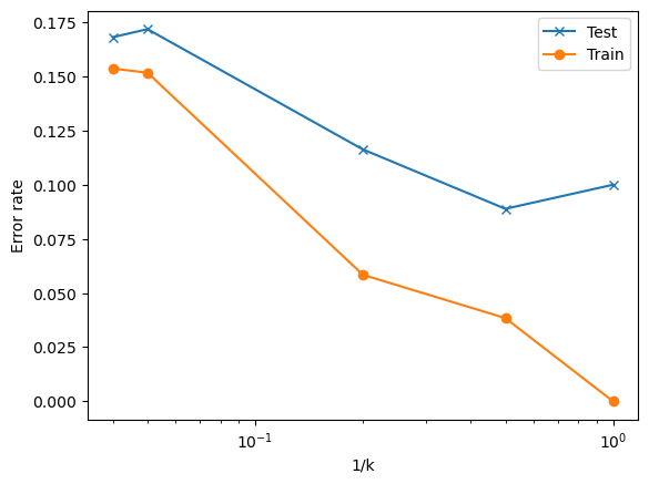
✅ Q: Based on your graph above
What do you notice about the shape of the train and test error plots?
What would you choose for \(k\) based on this data?
####YOUR ANSWER HERE###
Congratulations, we’re done!#
Initially created by Dr. Liz Munch, modified by Dr. Lianzhang Bao and Dr. Firas Khasawneh, Michigan State University

This work is licensed under a Creative Commons Attribution-NonCommercial 4.0 International License.