Jupyter Notebook

Lec 18: The Lasso

In this module we are going to test out the lasso method, discussed in class.

# Everyone's favorite standard imports
import numpy as np
import pandas as pd
import matplotlib.pyplot as plt
%matplotlib inline
import time


# ML imports we've used previously
from sklearn.model_selection import train_test_split
from sklearn.metrics import mean_squared_error
from sklearn.preprocessing import StandardScaler
from sklearn.linear_model import Ridge, RidgeCV
from sklearn.pipeline import make_pipeline


# Fix for deprecation warnings, but we should fix so this isn't here
import warnings 
warnings.filterwarnings('ignore')

Loading in the data

Ok, here we go, let’s play with a baseball data set again. Note this cleanup is all the same as the last lab.

url ="https://msu-cmse-courses.github.io/CMSE381-S26/_downloads/7c9ee5baa268e98bd5a1cade1809d7fe/Hitters.csv"
hitters_df = pd.read_csv(url)

# Print the dimensions of the original Hitters data (322 rows x 20 columns)
print("Dimensions of original data:", hitters_df.shape)

# Drop any rows the contain missing values, along with the player names
hitters_df = hitters_df.dropna().drop('Player', axis=1)

# Replace any categorical variables with dummy variables
hitters_df = pd.get_dummies(hitters_df, drop_first = True)

hitters_df.head()

Dimensions of original data: (322, 21)

	AtBat	Hits	HmRun	Runs	RBI	Walks	Years	CAtBat	CHits	CHmRun	CRuns	CRBI	CWalks	PutOuts	Assists	Errors	Salary	League_N	Division_W	NewLeague_N
1	315	81	7	24	38	39	14	3449	835	69	321	414	375	632	43	10	475.0	True	True	True
2	479	130	18	66	72	76	3	1624	457	63	224	266	263	880	82	14	480.0	False	True	False
3	496	141	20	65	78	37	11	5628	1575	225	828	838	354	200	11	3	500.0	True	False	True
4	321	87	10	39	42	30	2	396	101	12	48	46	33	805	40	4	91.5	True	False	True
5	594	169	4	74	51	35	11	4408	1133	19	501	336	194	282	421	25	750.0	False	True	False

y = hitters_df.Salary

# Drop the column with the independent variable (Salary)
X = hitters_df.drop(['Salary'], axis = 1).astype('float64')

X.info()

<class 'pandas.core.frame.DataFrame'>
Index: 263 entries, 1 to 321
Data columns (total 19 columns):
 #   Column       Non-Null Count  Dtype  
---  ------       --------------  -----  
 0   AtBat        263 non-null    float64
 1   Hits         263 non-null    float64
 2   HmRun        263 non-null    float64
 3   Runs         263 non-null    float64
 4   RBI          263 non-null    float64
 5   Walks        263 non-null    float64
 6   Years        263 non-null    float64
 7   CAtBat       263 non-null    float64
 8   CHits        263 non-null    float64
 9   CHmRun       263 non-null    float64
 10  CRuns        263 non-null    float64
 11  CRBI         263 non-null    float64
 12  CWalks       263 non-null    float64
 13  PutOuts      263 non-null    float64
 14  Assists      263 non-null    float64
 15  Errors       263 non-null    float64
 16  League_N     263 non-null    float64
 17  Division_W   263 non-null    float64
 18  NewLeague_N  263 non-null    float64
dtypes: float64(19)
memory usage: 41.1 KB

Finally, here’s a list of \(\alpha\)’s to test for our Lasso.

# List of alphas
alphas = 10**np.linspace(4,-2,100)*0.5
alphas

array([5.00000000e+03, 4.34874501e+03, 3.78231664e+03, 3.28966612e+03,
       2.86118383e+03, 2.48851178e+03, 2.16438064e+03, 1.88246790e+03,
       1.63727458e+03, 1.42401793e+03, 1.23853818e+03, 1.07721735e+03,
       9.36908711e+02, 8.14875417e+02, 7.08737081e+02, 6.16423370e+02,
       5.36133611e+02, 4.66301673e+02, 4.05565415e+02, 3.52740116e+02,
       3.06795364e+02, 2.66834962e+02, 2.32079442e+02, 2.01850863e+02,
       1.75559587e+02, 1.52692775e+02, 1.32804389e+02, 1.15506485e+02,
       1.00461650e+02, 8.73764200e+01, 7.59955541e+01, 6.60970574e+01,
       5.74878498e+01, 5.00000000e+01, 4.34874501e+01, 3.78231664e+01,
       3.28966612e+01, 2.86118383e+01, 2.48851178e+01, 2.16438064e+01,
       1.88246790e+01, 1.63727458e+01, 1.42401793e+01, 1.23853818e+01,
       1.07721735e+01, 9.36908711e+00, 8.14875417e+00, 7.08737081e+00,
       6.16423370e+00, 5.36133611e+00, 4.66301673e+00, 4.05565415e+00,
       3.52740116e+00, 3.06795364e+00, 2.66834962e+00, 2.32079442e+00,
       2.01850863e+00, 1.75559587e+00, 1.52692775e+00, 1.32804389e+00,
       1.15506485e+00, 1.00461650e+00, 8.73764200e-01, 7.59955541e-01,
       6.60970574e-01, 5.74878498e-01, 5.00000000e-01, 4.34874501e-01,
       3.78231664e-01, 3.28966612e-01, 2.86118383e-01, 2.48851178e-01,
       2.16438064e-01, 1.88246790e-01, 1.63727458e-01, 1.42401793e-01,
       1.23853818e-01, 1.07721735e-01, 9.36908711e-02, 8.14875417e-02,
       7.08737081e-02, 6.16423370e-02, 5.36133611e-02, 4.66301673e-02,
       4.05565415e-02, 3.52740116e-02, 3.06795364e-02, 2.66834962e-02,
       2.32079442e-02, 2.01850863e-02, 1.75559587e-02, 1.52692775e-02,
       1.32804389e-02, 1.15506485e-02, 1.00461650e-02, 8.73764200e-03,
       7.59955541e-03, 6.60970574e-03, 5.74878498e-03, 5.00000000e-03])

Lasso

Thanks to the wonders of scikit-learn, now that we know how to do all this with ridge regression, translation to lasso is super easy.

• Lasso Documentation

• LassoCV Documentation

• User guide

from sklearn.linear_model import Lasso, LassoCV

Here’s an example computing the lasso regression.

a = 1 #<------ this is me picking an alpha value

# normalize the input
transformer = StandardScaler().fit(X)
# transformer.set_output(transform = 'pandas') #<---- some older versions of sklearn
                                               #      have issues with this
X_norm = pd.DataFrame(transformer.transform(X), columns = X.columns)

# Fit the regression
lasso = Lasso(alpha = a) 
lasso.fit(X_norm, y)

# Get all the coefficients
print('intercept:', lasso.intercept_)
print('\n')
print(pd.Series(lasso.coef_, index = X_norm.columns))
print('\nTraining MSE:',mean_squared_error(y,lasso.predict(X_norm)))

intercept: 535.9258821292775


AtBat         -281.117268
Hits           303.712775
HmRun           11.130509
Runs           -25.237507
RBI             -0.000000
Walks          120.835970
Years          -35.043287
CAtBat        -161.321987
CHits            0.000000
CHmRun          14.271823
CRuns          375.151758
CRBI           192.215411
CWalks        -190.239127
PutOuts         78.676450
Assists         41.885267
Errors         -18.834451
League_N        23.209008
Division_W     -58.234428
NewLeague_N     -4.941839
dtype: float64

Training MSE: 92609.01554579365

And the version using the make_pipeline along with the StandardScaler function which gives back the same answer.

a = 1#<------ this is me picking an alpha value


# The make_pipeline command takes care of the normalization and the 
# Lasso regression for you. Note that I am passing in the un-normalized
# matrix X everywhere in here, since the normalization happens internally.
model = make_pipeline(StandardScaler(), Lasso(alpha = a))
model.fit(X, y)
 
# Get all the coefficients. Notice that in order to get 
# them out of the ridge portion, we have to ask the pipeline 
# for the specific bit we want with the model.named_steps['ridge']
# in place of just ridge from above.
print('intercept:', model.named_steps['lasso'].intercept_)
print('\n')
print(pd.Series(model.named_steps['lasso'].coef_, index = X.columns))
print('\nTraining MSE:',mean_squared_error(y,model.predict(X)))

intercept: 535.9258821292775


AtBat         -281.117268
Hits           303.712775
HmRun           11.130509
Runs           -25.237507
RBI             -0.000000
Walks          120.835970
Years          -35.043287
CAtBat        -161.321987
CHits            0.000000
CHmRun          14.271823
CRuns          375.151758
CRBI           192.215411
CWalks        -190.239127
PutOuts         78.676450
Assists         41.885267
Errors         -18.834451
League_N        23.209008
Division_W     -58.234428
NewLeague_N     -4.941839
dtype: float64

Training MSE: 92609.01554579365

✅ Do this: Mess with the values for \(a\) in the code, such as for \(a=1, 10, 100, 1000\). What do you notice about the coefficients?

Your answer here

✅ Do this: Make a graph of the coeffiencts from lasso as \(\alpha\) changes

Note: we did similar things in the last class but with ridge regression, so I’ve included the code you can borrow and modify from there. Also note I got a bunch of convergence warnings, but drawing the graphs I could safely ignore them. There’s a command you ran in the first box to ignore warnings so they might not show up at all.

# Your code for computing the coefficients goes here 
# I've included the code from last class that did this for the ridge version
# so you should just need to update it to do lasso instead.


coefs = []

for a in alphas:
    model = make_pipeline(StandardScaler(), Ridge(alpha = a))
    model.fit(X, y)
    coefs.append(model.named_steps['ridge'].coef_) #<--modify here
    

coefs = pd.DataFrame(coefs,columns = X_norm.columns)
coefs.head()
   

	AtBat	Hits	HmRun	Runs	RBI	Walks	Years	CAtBat	CHits	CHmRun	CRuns	CRBI	CWalks	PutOuts	Assists	Errors	League_N	Division_W	NewLeague_N
0	6.780624	7.846413	5.668981	7.382901	7.739614	7.908231	6.536754	8.894638	9.417447	8.959603	9.653524	9.732533	8.177650	5.941721	0.482213	-0.198173	0.147069	-4.066839	0.260218
1	7.482871	8.711141	6.222836	8.176418	8.547140	8.775630	7.167294	9.803256	10.402015	9.888785	10.662606	10.750886	8.995532	6.681835	0.538299	-0.238435	0.221313	-4.609158	0.332227
2	8.221672	9.637282	6.796229	9.020407	9.399342	9.703560	7.819084	10.758248	11.443720	10.869669	11.730158	11.828595	9.849605	7.497878	0.598915	-0.287508	0.315973	-5.215881	0.420140
3	8.991208	10.622778	7.382157	9.911172	10.290649	10.689638	8.484413	11.752906	12.537320	11.896678	12.850766	12.960326	10.732098	8.394523	0.664011	-0.347297	0.434733	-5.892882	0.526287
4	9.784056	11.664507	7.972138	10.843736	11.213981	11.730347	9.154123	12.779016	13.676264	12.962918	14.017662	14.139408	11.633564	9.376262	0.733471	-0.420043	0.581480	-6.646198	0.652960

# If that worked above, you'll get a graph in this code. 

for var in coefs.columns:
    # I'm greying out the ones that have magnitude below 200 to easier visualization
    if np.abs(coefs[var][coefs.shape[0]-1])<200:
        plt.plot(alphas, coefs[var], color = 'grey', linewidth = .5)
    else:
        plt.plot(alphas, coefs[var], label = var)

plt.xscale('log')
plt.axis('tight')
plt.xlabel('alpha')
plt.ylabel('coefficients')

plt.legend()

<matplotlib.legend.Legend at 0x12fa252d0>

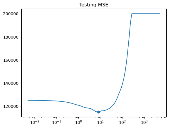
✅ Do this: Make a graph the test mean squared error as \(\alpha\) changes for a fixed train/test split.

Note: again I’ve included code from last time that you should just have to update.

# Update this code to get the MSE for lasso instead of Ridge
X_train, X_test , y_train, y_test = train_test_split(X, y, test_size=0.3, random_state=1)

errors = []

for a in alphas:
    model = make_pipeline(StandardScaler(), Ridge(alpha = a)) #<--modify here
    model.fit(X_train, y_train)

    pred = model.predict(X_test)
    errors.append(mean_squared_error(y_test, pred))

# If that worked, you should see your test error here.
i = np.argmin(errors) # Index of minimum 
print(f'Min occurs at alpha = {alphas[i]:.2f}')
print(f'Min MSE is {errors[i]:.2f}')

plt.title('Testing MSE')
plt.plot(alphas,errors)
plt.scatter(alphas[i],errors[i])
ax=plt.gca()
ax.set_xscale('log')

Min occurs at alpha = 8.15
Min MSE is 115059.67

✅ Do this: make a plot showing the number of non-zero coefficients as a function of the \(\alpha\) choice.

Hint: I used the np.count_nonzero command on the coefs data frame we already built

# Your code here

✅ Q: Say your goal was to end up with a model with 5 variables used. What choice of \(\alpha\) gives us that and what are the variables used?

# Your code here 

Lasso with Cross Validation

✅ Do this: Now try what we did with LassoCV. What choice of \(\alpha\) does it recommend?

I would actually recommend either not passing in any \(\alpha\) list or passing explicitly alphas = None. RidgeCV can’t do this, but LassoCV will automatically try to find good choices of \(\alpha\) for you.

# Here's the ridge code from last time that you should update

X_train, X_test , y_train, y_test = train_test_split(X, y, test_size=0.3, random_state=1)

# To make sure my normalization isn't snooping, I fit the transformer only 
# on the training set 
transformer = StandardScaler().fit(X_train)
# transformer.set_output(transform = 'pandas')
X_train_norm = pd.DataFrame(transformer.transform(X_train), columns = X_train.columns)

# but in order for my output results to make sense, I have to apply the same 
# transformation to the testing set. 
X_test_norm = transformer.transform(X_test)

# I'm going to drop that 0 from the alphas because it makes 
# RidgeCV cranky
alphas = alphas[:-1]


ridgecv = RidgeCV(alphas = alphas, 
                  scoring = 'neg_mean_squared_error', 
                  )
ridgecv.fit(X_train_norm, y_train)

print('alpha chosen is', ridgecv.alpha_)

alpha chosen is 1.5269277544167077

# Your code here

Now let’s take a look at some of the coefficients.

# Some of the coefficients are now reduced to exactly zero.
pd.Series(lassocv.coef_, index=X.columns)

AtBat         -328.601267
Hits           351.501357
HmRun          -28.435135
Runs           -48.625331
RBI             56.256350
Walks          124.840026
Years           -0.000000
CAtBat        -368.328399
CHits          365.286546
CHmRun         143.047744
CRuns          128.855535
CRBI            70.376722
CWalks        -143.423781
PutOuts         93.738170
Assists          9.972723
Errors           0.274326
League_N         8.803090
Division_W     -60.734020
NewLeague_N      9.219834
dtype: float64

✅ Q: We’ve been repeating over and over that lasso gives us coefficients that are actually 0. At least in my code, I’m not seeing many that are 0. What happened? Can I change something to get more 0 entries?

###Your answer here###You might also want some code in here to try to figure it out

---

Congratulations, we’re done!

Initially created by Dr. Liz Munch, modified by Dr. Lianzhang Bao and Dr. Firas Khasawneh, Michigan State University

This work is licensed under a Creative Commons Attribution-NonCommercial 4.0 International License.