Homework 3: Modeling the Lorenz system and designing a compartmental model

Homework 3: Modeling the Lorenz system and designing a compartmental model#

✅ Put your name here.#

Goals#

In this homework, you will use Numpy, SciPy and Matplotlib to model the Lorenz system. This should serve as a good assessment of what you understand at this point in the course. Make sure to use Teams and help room hours if you run into issues!

By the end of the homework assignment you will have practiced:#

Using solve_ivp to solve a set of ODEs for the purposes of modeling a phenomenon
Using matplotlib to visualize models
Building compartmental models
Interpreting model results

Assignment instructions#

Work through the following assignment, making sure to follow all of the directions and answer all of the questions.

This assignment is due at 11:59pm on Friday, March 8th. It should be uploaded into the “Homework Assignments” dropbox folder for Homework #3. Submission instructions can be found at the end of the notebook.

Grading#

Part 1: Lorenz system (42 points)
Part 2: Compartment model (12 points)

Total points possible: 55

Part 1: Lorenz system (42 points)#

The Lorenz system is a system of ordinary differential equations first studied by mathematician and meteorologist Edward Lorenz, who was trying to understand why weather prediction is inherently so difficult to predict very far out. It is notable for having chaotic solutions for certain parameter values and initial conditions. In particular, the Lorenz attractor is a set of chaotic solutions of the Lorenz system. In popular media the “butterfly effect” stems from the real-world implications of the Lorenz attractor, namely that in a chaotic physical system, in the absence of perfect knowledge of the initial conditions (even the minuscule disturbance of the air due to a butterfly flapping its wings), our ability to predict its future course will always fail.

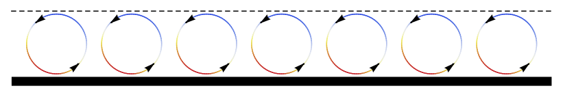
Let’s try to get a grip on what the Lorenz attractor really is. To get to the crux of the issue, Dr. Lorenz did what many scientists do - he drastically simplified. In many ways, the atmosphere behaves like a fluid so he studied the simplest fluid with interesting dynamics he could think of - a pot of slowly heating water. As the water is heateded slowly, convection rolls begin. The situation might look something like so.

According to Lorenz, there are three quantities that characterize the state of the weather:

x: the rate of convective motion - i.e. how fast the rolls are rotating,
y: the temperature difference between the ascending and descending currents, and
z: the distortion (from linearity) of the vertical temperature profile.

Lorenz showed that the above three quantities are related via a set of ordinary differential equations (ODEs)

\begin{equation*} \begin{aligned} \frac{\mathrm{d}x}{\mathrm{d}t} &= \sigma (y - x), \[6pt] \frac{\mathrm{d}y}{\mathrm{d}t} &= x (\rho - z) - y, \[6pt] \frac{\mathrm{d}z}{\mathrm{d}t} &= x y - \beta z, \end{aligned} \end{equation*}

where \(\sigma\), \(\rho\), and \(\beta\) are system parameters. Your goal is now to understand this model by using solve_ivp to solve it with different initial conditions and parameters. In order to deepen your knowledge in this field, you now want to initiate yourself to the modeling of the above Lorenz system.

Part 1.1: Preliminary (1 point)#

✅ Question 1.1 (1 point):#

Make sure you set up your notebook to import the right modules that you will need in this homework. You may need to look through the assignment first, in order to get a sense for what you might need to use.

# Put your code here

Part 1.2: Find a numerical solution of the Lorenz model (27 points)#

As a first step, let us find an approximation of the solution of the Lorenz model for a given initial condition for \(x\), \(y\), and \(z\).

✅ Question 1.2 (5 points):#

Construct a model of the Lorenz system by defining the derivative function named deriv_lorenz for the above ODEs (\(\frac{\mathrm{d}x}{\mathrm{d}t}\), \(\frac{\mathrm{d}y}{\mathrm{d}t}\), \(\frac{\mathrm{d}z}{\mathrm{d}t}\)) with input such as t, curr_val, sigma, rho, beta.

# Put your code here

✅ Question 1.3 (12 points):#

Compute the prediction of \(x\), \(y\), and \(z\) for a time interval of \([0,50]\) using solve_ivp with the timestep \(dt = 0.02\), initial condition \(x_0 = 6\), \(y_0=6\), \(z_0=8\), and parameters \(\sigma = 10\), \(\rho = 28\), \(\beta = 8/3\). Make three plots for the evolution of \(x\), \(y\), and \(z\), respectively. You should end up with plots that look similar to this:

# Put your code here

✅ Question 1.4 (7 points):#

Make a 3D Visualization of the solution for \(x\), \(y\), and \(z\) by completing the code include below or by writing your own code from scratch, whichever option makes more sense to you. You are expected to get 3D plot similar to the following “butterfly” pattern (not exactly the same). Once you make your plot, describe what you observe in the provided markdown cell below.

# Hint: If you want, you can modify the following code to make this plot, or you can use an approach that you prefer
# There are pieces missing from this code and things that you need to alter to make it work with the code you've already written,
# but it should give you an idea of how to plot the 3D trajectory and create a dot at each point

#fig = plt.figure(figsize=(8,8))
#ax = fig.add_subplot(111, projection="3d")
#for i in range():
#    ax.scatter(x, y, z, s=2)

#ax.plot3D(x,y,z, 'gray')

# Put your code here

✎ Describe what you observe here.

✅ Question 1.5 (3 points):#

Re-run the model of the same initial condition \(x_0 = 6\), \(y_0=6\), and \(z_0=8\) but with different parameters \(\sigma = 28\), \(\rho = 10\), \(\beta = 8/3\). Make the 3D plot. What do you observe for this case (put your response in the markdown cell provide following your plot)?

# Put your code here

✎ Describe what you observe.

Part 1.3: Prediction with different initial conditions (14 points)#

✅ Question 1.6 (8 points):#

Now that we have a functional model, we are going to explore how the results of the model change as we vary the initial conditions, even for small changes.

Let us create a function named compare_parameters that takes the following input arguments: init1 and init2, which are two different initial conditions, and sigma, rho, beta which, as before, are the model parameters. The function should plot 3 figures. Each plot should be the predicted \(x\), \(y\), \(z\) for a time interval of \([0,10]\) for the two different sets of initial values, respectively. (Your resulting plots should look similar to Question 3, but there should be two lines on each plot for the two different sets of initial values).

# Put your code here

✅ Question 1.7 (6 points):#

Now that you’re written your function, you’re going try to experiment with this function for parameter values from the previous parts of the assignment (i.e. \(\sigma = 10\), \(\rho = 28\), \(\beta = 8/3\); and \(\sigma = 28\), \(\rho = 10\), \(\beta = 8/3\)). You can set init1=[6, 6, 8] and init2=[6.1, 6.1, 8.1] in this case (which means init2 is a small perturbation of init1) and predict \(x(t)\), \(y(t)\), and \(z(t)\) for a time interval of \([0,10]\). Your code should call your compare_parameters function twice and generate two sets of \(x\), \(y\), \(z\) plots.

What difference do you observe? Which parameter values are more sensitive to the small change in the initial values? Record your answers to these questions in the markdown cell below.

# Put your code here

✎ Describe what you observe.

Part 2: Compartment model in Chemistry (12 points)#

An amount of sodium chloride \(\textrm{NaCl}\) is poured into a bucket with clean water. In this solution sodium chloride is transfered to \(\textrm{Na}^+\) and \(\textrm{Cl}^-\) with a rate \(k_1\). At the same time \(\textrm{Na}^+\) reacts with \(\textrm{Cl}^-\) to form \(\textrm{NaCl}\) with a rate \(k_2\). If you want more information, part of the process is described in the video linked below.

from IPython.display import YouTubeVideo
YouTubeVideo("8g-qdC1McBk",width=640,height=360)

In this example, the basic reaction that is occurring is that the \(\textrm{NaCl}\), which is a solid salt, is interacting with the water and dissolving to form free \(\textrm{Na}^+\) and \(\textrm{Cl}^-\) ions. The water itself isn’t actually changing, it’s just acting as the mechanism for breaking the salt into it’s separate ions. While the salt is being dissolved in the water, there are also natural reactions taking place in which the \(\textrm{Na}^+\) and \(\textrm{Cl}^-\) ions are recombining to form salt (which is why, if you leave the salty water out and it evaporates, you would see the solid salt reform).

And remember, in this reaction, sodium chloride, \(\textrm{NaCl}\), is transfered to \(\textrm{Na}^+\) and \(\textrm{Cl}^-\) with a rate \(k_1\). At the same time \(\textrm{Na}^+\) reacts with \(\textrm{Cl}^-\) to form \(\textrm{NaCl}\) with a rate \(k_2\).

✅ Question 2.1 (8 points)#

Your job is to design and draw a compartment model for this chemical process. You can take a picture of your model and insert it as an image. Here is a link on how to insert image in the notebook.

To facilitate the modeling process, you should answer the following questions first.

How many compartments are needed in the model?
- Since we are ignoring the effects from water, i.e. water evaporation, is it necessary to consider water as a compartment?
- What is the relationship between the amount of \(\textrm{Na}^+\) and \(\textrm{Cl}^-\)?

✎ Answer the questions. Put a diagram of your compartment model here.

✅ Question 2.2 (4 points)#

Based on the diagram (or model you formulated) above, write down a set of equations that accurately represent your model.

✎ Write your equations here.

Congratulations, you’re done!#

Submit this assignment by uploading it to the course Desire2Learn web page. Go to the “Homework Assignments” folder, find the dropbox link for Homework #3, and upload it there.