Day 22 In-class Assignment: Random Walks

Day 22 In-class Assignment: Random Walks#

✅ Put your name here.
#

✅ Put your group member names here.
#

Goals for today’s In-Class assignment#

Model a random walk
Learn about the behavior of random walks in one and two dimensions
Plot both the distribution of random walks and the outcome of a single random walk

Assignment instructions#

Work with your group to complete this assignment. Instructions for submitting this assignment are at the end of the notebook. The assignment is due at the end of class.

Random Walks: What and Why?#

Random walks are a great first step towards modeling dynamical systems in which there is a random component. Here we will use our knowledge of loops and if-statements to run random walk simulations, study their properties, and connect them to the Einstein diffusion relation. But, random walks like this are used to model a wide range of systems, including financial markets, biochemical reaction networks, atomic-scale motions, and much more.

In many situations, it is very useful to think of processes with randomness as a succession of random steps. This can describe a wide variety of phenomena - the behavior of the stock market, models of population dynamics in ecosystems, the properties of polymers, the movement of molecules in liquids or gases, modeling neurons in the brain, or in building Google’s PageRank search model. This type of model is known as a “random walk”, and while the process being modeled can vary tremendously, the underlying process is simple. In this project, we are going to model such a random walk and learn about some of its behaviors!

Historical Background and Einstein’s Relation#

Brown

Random walks are sometimes referred to as Brownian motion, which referred originally to the motions of a single grain of pollen suspended in a liquid solution. It is named after Robert Brown, who studied pollen under a microscope in 1829 in an attempt to understand the reproductive process in plants. But in fact a little Wikipedia-ing reveals this phenomenon has been documented much earlier. An excerpt from a poem by Lucreitus in 60 BC is remarkably on point:

“Observe what happens when sunbeams are admitted into a building and shed light on its shadowy places. You will see a multitude of tiny particles mingling in a multitude of ways… their dancing is an actual indication of underlying movements of matter that are hidden from our sight… It originates with the atoms which move of themselves [i.e., spontaneously]. Then those small compound bodies that are least removed from the impetus of the atoms are set in motion by the impact of their invisible blows and in turn cannon against slightly larger bodies. So the movement mounts up from the atoms and gradually emerges to the level of our senses, so that those bodies are in motion that we see in sunbeams, moved by blows that remain invisible.”

This remained surprisingly challenging to understand until Einstein in 1905, who rigorously tied the motion of the large particles (e.g. pollen) to the motions of many atoms (e.g., the water molecules the pollen was in). What Brown saw under his microscope was a jiggling pollen grain, and Einstein showed that the jitter was due to many rapid collisions with water molecules. See the animation above.

A prediction of Einstein is the “Einstein diffusion relation” (here, in 3 dimensions):

\( \left< \left(r(t)-r(0)\right)^2\right> = 6Dt\)

where \(r(t)\) is the position of a particle at time \(t\), \(D\) is the diffusion coefficient, and the angle brackets denote an average over an ensemble of measurements.

What does this mean? We measure the distance from the particle’s initial position, \(r(0)\), which is \(|r(t) - r(0)|\), over many different experiments and find that the mean squared distance (defined in the angle brackets above) increases linearly with time. You might ask: is that so surprising? It is when you consider the fact that Brown could not see the water molecules in his microscope, so the motion might be predicted to be given by \(r = vt\), which predicts an increase in time of the squared distance of \(t^2\); because the particle under observation (pollen in this case) can reverse directions over and over, its distance from the origin increases more slowly as just \(t\). The slope is the diffusion coefficient. (This could be people buying and selling a stock over and over.)

Today we are going to code random walks and test their ability to model the behavior of diffusive particles.

Part 1: One-dimensional random walk.#

Let’s start with the simplest case: a 1D random walk; that is, a random walk on a line.

Imagine that you draw a line on the floor, with a mark every foot. You start at the middle of the line (the point you have decided is the “origin”, at \(x=0\)). You then flip a “fair” coin \(N\) times (“fair” means that it has equal chances of coming up heads and tails). Every time the coin comes up heads, you take one step to the right (in the + direction). Every time it comes up tails, you take a step to the left (in the - direction).

The questions we’re going to answer:

After \(N_{step}\) coin flips and steps, how far are you from the origin?
If you repeat this experiment \(N_{trial}\) times, what will the distribution of distances from the origin be, and what is the mean distance that you go from the origin? (Note: “distance” means the absolute value of distance from the origin!)

First: as a group, come up with a solution to this coding problem on your whiteboard. Use a flow chart, pseudo-code, diagrams, or anything else that you need to get started. Check with an instructor before you continue! Make sure you come up with a plan for not only how you are going to code your random walk, but how you will keep track of every new trial/walk you run.

Note: Once you’ve drafted your plan, we’re going to pursue one possible path toward a solution in the rest of the notebook, this may be different than how you planned it out. If this is the case, think about how the content below compares to the plan you came up with and reflect on which option you like more and why.

🛑 STOP#

Check in with an instructor before moving on! Talk them through your plan!

Coding up a solution#

✅ Do This: After checking in with your instructors: In pairs, write a function, called step1d, that uses a random number generator to return instructions to take a step either left or right, which means that it should return -1 or +1. Call the function a few times and print out the value it returns to make sure it works - we’ll use this as the basis of our random walk model.

Check with other pairs at your table to compare their method for writing the step function to yours.

import numpy as np
import random
import matplotlib.pyplot as plt
%matplotlib inline

import seaborn as sns

sns.set_context('notebook')

# put your code here.

✅ Do This: Now, as a group write a code in the space provided below to do a single random walk with \(N_{step} = 1000\) using the function you have created. You’ll start at \(x=0\) and take \(N_{step}\) consecutive steps to the right or left. At the end print the value of \(x\). Where did your particle go? Run it a couple of times to see how this changes.

# put your code here.

Okay, great! But, it would be much better if we could visualize what is happening.

✅ Do This: Copy the code from above and modify it to keep track of the number of each step and your distance from the origin, and plot it!

(Hint: start with empty arrays or lists, and append to them.) Run this a couple of times to see how it changes. You should get something that ends up looking like this:

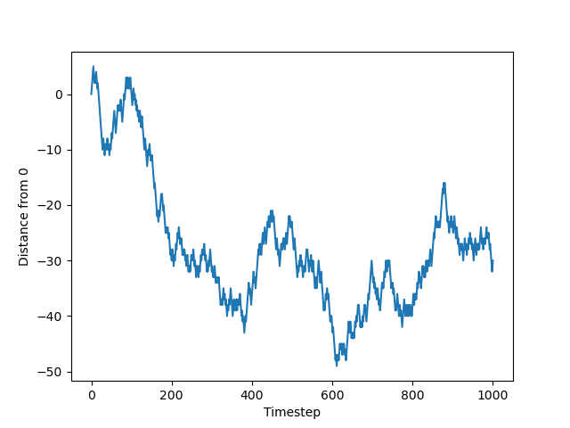
Don’t forget to label your axis.

Advanced: If you save the path of your particle as all_x, the code below will animate the random walk for you.

# put your code here.

# If you save your walk as `all_x`, you can run the following code to animate it.
import time
from IPython.display import clear_output

max_frames_in_animation = 100 # change this for longer or shorter animation

fig = plt.figure(figsize=(6,1))

for i in range( min( len(all_x), max_frames_in_animation)):

    plt.scatter(all_x[:i], np.zeros_like(all_x[:i]), color = 'grey')
    plt.scatter(all_x[i+1], [0], color = 'red', s = 100)

    plt.title('The current value of i is: '+ str(i))
    plt.xlim(-15,15)
    plt.ylim(-1,1)
    time.sleep(1)  
    clear_output(wait = True)
    display(fig)            # Reset display
    fig.clear()             # clear output for animation

Now, we want to see how several of these trajectories look at the same time.

✅ Do This: Copy and paste your code from above and add an additional loop where you make five separate trajectories, and plot each of them on the same plot. There is more than one way that you could do this. You could store the trajectories using a 2D array or by creating a list composed of lists of trajectories. Alternatively, you could all call the plot command within your loop and avoid storing the trajectories completely. The structure of the code is up to you!

# put your code here.

✅ Do This: Ok. Now we’re getting somewhere. Let’s increase the number of trajectories from 5 to 1000. But what about all the memory that will be required to store that many trajectories? Let’s be nice to our computers and not make them keep track of every single walk, just the final points. So, after copying and pasting your code from above, comment out the code that either saved the trajectories or plotted every walk and instead just store the final position from every random walk in a new list.

Once you have code that stores all of the final positions, calculate \(\left< \left |r(t)-r(0)\right |^2\right>\), which is the equation from above and is the average squared distance of the walk. What is \(r(0)\) in this case? (Note: we’re keeping track of average squared distance because that makes it easier to do the next part!)

Also, plot a histogram of the final distances.

Hint: You may want to use a numpy array and append distances to it, then you can square the values in the array and compute the mean of those values using the NumPy function. Look at the help for np.append()! Alternatively, you can store the values in a list and then convert them to a NumPy array using np.array().

# put your code here.

We’re almost ready for Einstein! All we have to do is add another layer to our loop structure. We want to see how far the particle goes, on average, as a function of the number of steps (which is actually just a proxy for time, since the size of the time steps are all the same).

✅ Do This: Extend the code you wrote above to get the average of the square of the final position at 10 different time points (t = 100, 200, …, 1000), and save the results to a list. Plot the results versus time below, and use axis labels.

# put your code here.

# make plot here

✅ Question: Looking at the above plot, is this what you would have expected from the Einstein diffusion equation? Why or why not?

Put your answer here!

Part 2: (Time-permitting) Two-dimensional walk#

Now, we’re going to do the same thing, but in two dimensions, x and y. This time, you will start at the origin, pick a random direction (up, down, left, or right), and take one step in that direction. You will then randomly pick a new direction, take a step, and so on, for a total of \(N_{step}\) steps.

Questions:

After \(N_{step}\) random steps, how far are you from the origin?
If you repeat this experiment \(N_{trial}\) times, what will the distribution of distances from the origin be, and what is the mean distance that you go from the origin? (Note: “distance” means the absolute value of distance from the origin!) Does the mean value differ from Part 1?
For one trial, plot out the steps taken in the x-y plane. Does it look random?

First: As before, come up with a solution to this problem on your whiteboard as a group. Check with an instructor before you continue!

Then: In pairs, write a code in the space provided below to answer these questions! (Hint: Start by modifying your coin-flip code to return an integer that is 0,1,2, or 3 (left, right, up, down). How do you modify your function?)

✅ Do This: As above, loop over this, but this time use the following rule: (0 => go left, 1 => go right, 2 => go up, 3 => go down). Start at x=0,y=0, and run for 1000 steps, while keeping track of the trajectory. Plot the result as x versus y. Do this a few times and see how it changes! (Again, if you want to try to animate this, see the code example at the end of this notebook.)

✅ Do This: Now plot the x and y values versus time, individually.

✅ Do This: How do these curves compare to the results of your 1D random walk?

Answer here:

✅ Question: Recall the Einstein equation for 3 dimensions: \(\left<(r(t)-r(0))^2\right> = 6Dt\). Given that \(r(0) = 0\) and that \(r^2 = x^2 + y^2 + z^2\). What do you think the corresponding Einstein equations are for 1D and 2D?

Answer here:

Congratulations, we’re done!#

Now, you just need to submit this assignment by uploading it to the course Desire2Learn web page for today’s submission folder (Don’t forget to add your names in the first cell).

Animation Code#

It can be interesting to animation your random walk so that you can watch it move about as it makes its walk. If you have the time, you can try this. Below is a code snippet that you’ve probably seen before earlier in the course, but it’s incuded here so that you can try to use it for this problem!

# make sure things like NumPy and matplotlib are imported before trying this

# other important imports
import time
from IPython.display import clear_output

fig = plt.figure(figsize=(12,9))

x_hold = []
y_hold = []

for i in range(100):
    x = np.random.random()
    y = np.random.random()
    x_hold.append(x)
    y_hold.append(y)
    plt.plot(x_hold,y_hold,'ro')
    print('The current value of i is:', i)
    plt.xlim(0,1)
    plt.ylim(0,1)
    time.sleep(0.1)  
    clear_output(wait = True)
    display(fig)            # Reset display
    fig.clear()             # clear output for animation