Day 8: In-class Assignment: Introduction to Modeling with ODEs#
✅ Put your name here.
#✅ Put your group member names here.
#
Goals for Today’s In-Class Assignment#
By the end of this assignment, you should be able to:
Use Python to numerically solve an ordinary differential equation (ODE)
Apply numerical integration to model population growth over time
Visualize how the population changes over time by making plots
Explore other ODE models
Assignment instructions#
Today, with your group, you’re going to try to apply what you’ve learned in the pre-class assignment to explore modeling with ordinary differential equations.
This assignment is due at the end of class and should be uploaded into the appropriate “In-class Assignments” submission folder. Submission instructions can be found at the end of the notebook.
Part 0: What were we doing again?#
Recall from the video that the ordinary differential equation describing population is:
\begin{equation} \frac{dP}{dt} = kP\Big(1-\frac{P}{C}\Big), \end{equation}
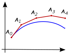
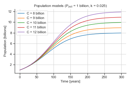
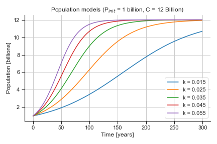
where \(P =\) population, \(k =\) growth rate, and \(C =\) the carrying capacity. If we make our initial population be 1 billion and vary the other parameters, the solution \(P(t)\) looks like the figures below.
Part 1: Reviewing Observations from the Pre-class#
✅ 1.1 Task#
As a group, discuss your answers to Parts 3 and 4 of the pre-class. Summarize your discussion below. For the population model, what parameters are changing and which are not? What differences did you have in your responses?
✎ Put your answer here
✅ 1.2 Task#
As a group, compare your derivs functions and your pseudocode for update equations. Determine how you as a group would combine derivs and the update equations loop to solve an ODE. In the cell below, summarize your discussion.
✎ Put your answer here
STOP#
Discuss your pseudocode for with an instructor before moving on!
Part 2: Coding Update Equations#
✅ 2.1 Task#
In the cell below, fill in the derivs function with the code you agreed upon as a group.
# Define a function that computes the derivatives
✅ 2.2 Task#
To actually solve the ODE, you will need to code the update equations. Use your pseudo-code from the previous part to write an update equation that numerically integrates \(\frac{dP}{dt}\). Use the following values for your solution:
P0 = 1.0e9k=0.01C=1.2e10
Your code should result in a list (or array) of population values for the time interval from 0 to 500 years in steps of 50 years. Your solution must call your derivs function.
# Write your code here
✅ 2.3 Question#
How do you know your code is working? You’ll likely want to write a bit of code to confirm that it is working as intended! Put that code in the cell below.
# put your tests here
Part 3: Comparing Numerical Solution to Exact Solution#
✅ 3.1 Task#
What we have just done is a form of Numerical Integration. Numerical Integration is a way to approximate the integral of a differential equation, instead of the exact solution, which you get by taking the integral of \(\frac{dP}{dt}\).
The exact solution to the differential equation we’ve been working with is: $\(P(t) = \frac{C}{1 + Ae^{-k_R t}}\)\( Where \)\(A = \frac{C-P_{0}}{P_{0}}\)$ (We’ve actually worked with this equation before, when we first started making visualizations.)
Let’s compare the results of our numerical integration–which is an approximation–to the exact solution for \(P(t)\) given above. We’ve provided you with a function for calculating the exact solution below. Calculate \(P(t)\) using the exact solution.
def pop_func_exact_sol(time,pinitial,bigc,littlek):
    a = (bigc - pinitial)/pinitial
    pop = bigc/(1 + a*np.exp(-1.0*littlek*time))
    return pop
# Write your code for calculating P using the exact solution above
✅ 3.2 Task#
Make a single plot that shows your numerical solution from 2.2 along with the exact solution from the previous question. Make sure your plot include axes labels and a legend.
# Write your code for making a single plot showing your numerical solution vs the exact solution
✅ 3.3 Question#
How does the numerical integration solution compare to the exact solution? If your job involved modeling, would you feel confident using the results from the numerical solution?
✎ Put your answer here
Part 4: Changing the Time Step#
✅ 4.1 Task#
We mentioned previously that, with numerical integration, our results are approximate solutions. There are certain things that we can do to improve our approximation.
Repeat steps 2.2, 3.1, and 3.2 using a time step of 20 years. That is, use numerical integration to find approximate values for P and use the function from 3.1 to find exact values for P using the new time step, and then plot the values against each other.
# put your code here
✅ 4.2 Question#
What effect does changing the time step have on your numerical solution?
✎ Put your answer here
✅ 4.3 Question#
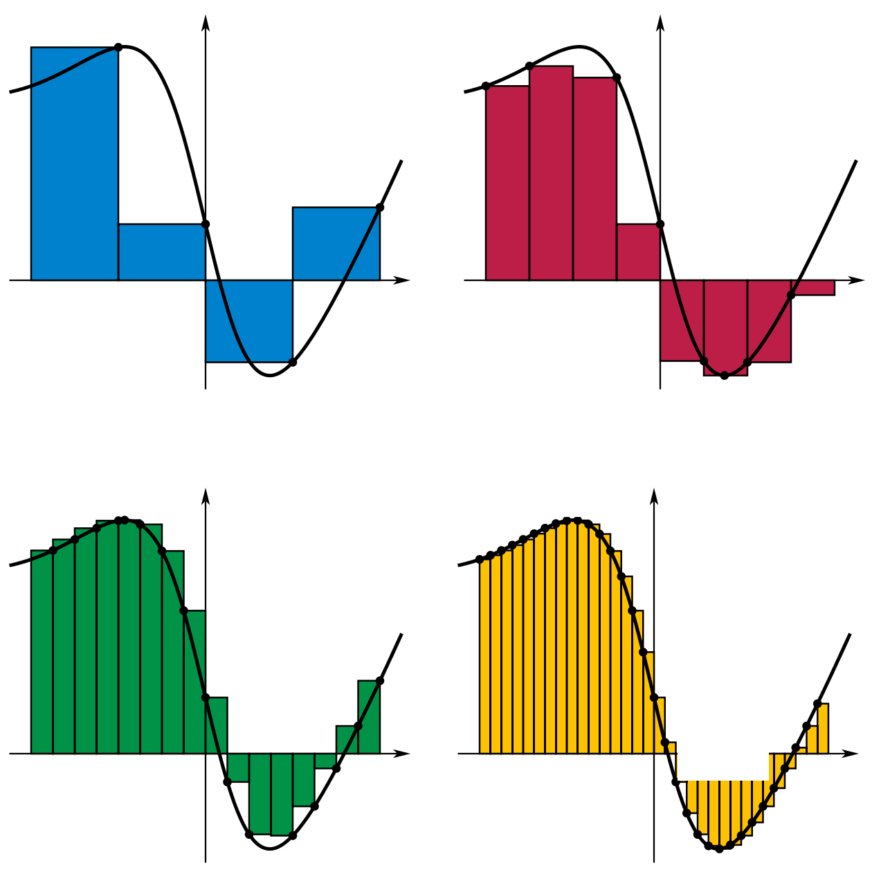
What we’ve been doing for our numerical integration is the same as taking the Riemann Sum, which involves calculating an integral by drawing little boxes (or other shapes) underneath a curve, calculating the area of each box, and summing them together.
Consider the following figure, which shows Riemann sums for different step sizes. Use this figure to explain why changing the time step affects your numerical solution. (Remember: Integration is basically finding the area under a curve!)
✎ Put your answer here
✅ 4.4 Question#
As you found in with your code and in looking at the image above, it seems like taking smaller and smaller steps leads to a more accurate solution. What is the trade-off to taking smaller steps? Are there reasons why we might need or want to take larger steps? How might be decide what step size is “good enough”?
✎ Put your answer here
Part 5 (Time Permitting): Exploring Another Model#
There are several other simple ordinary differential equations that have solutions we can obtain similarly to the population growth model. This website mentions a few of them.
✅ 5.1 Question#
Research one of the models on the website, and answer the following questions:
Describe the model and the system it is modeling.
What are the parameters that are changing?
What are the parameters that are constant?
What derivatives would you calculate in your
derivsfunction?
✎ Put your answer here
✅ 5.2 Task#
Write a new derivs function for your new model. Test it in the same way you tested the population growth model in the pre-class.
# put your code here
Congratulations, you’re done!#
Submit this assignment by uploading it to the course Desire2Learn web page. Go to the “In-Class Assignments” folder, find the appropriate submission link, and upload it there.
© Copyright 2023, Department of Computational Mathematics, Science and Engineering at Michigan State University.