Week 09: Pre-Class Assignment: ANN Playground#
✅ Put your name here.#
✅ Put your group member names here.
Goals for this week’s pre-class assignment#
In this Pre-Class Assignment you are going to use play around with neural networks in order to build your intuition of what they actually do.
Total number of points: 18 points (2 points per question)
This assignment is due by 11:59 p.m. the day before class, and should be uploaded into the appropriate “Pre-Class Assignments” submission folder on D2L. Submission instructions can be found at the end of the notebook.
Part 0: Reading#
Read chapters 10 and 11 of your textbook. Read through the questions at the end of each chapter and the answers in the Appendix.
Part 1: Neural Network Intuition#
All ML algorithms require you to make choices about how to use the algorithm:
the number of neighbors in kNN,
the choice and properties (e.g., width \(\sigma\)) of basis functions in RBFs,
regularization type (L1, L2, EN) and strength (\(\lambda\)),
and so on.
ANNs in particular have a large number of choices that you need to make, and it is not easy to know how to make those choices.
In this problem you are going to build your intuition about how to make such choices and explain this intuition. To do this, you will run a large number of ANNs with various datasets, with various inputs, for various depths, for various widths, observing the contents of the hidden layers, examining the optimization process and so on. You can’t really build your intuition for ANNs without spending a lot of time varying all of these choices together simulataneously. No pain, no gain.
Fortunately, there is an excellent web app for doing just this.
✅ Task: Go to this webpage. You will see a dashboard with:
choice of four datasets at the upper left,
below that you see training choices,
at the very right you can see the current output of the NN,
at the bottom right you can change what is being displayed - training versus testing, for example,
along the top you have controls for the regularization, activiation, learing rate and problem type,
note that if you switch the problem type to regression, the choice of datasets at the upper left changes.
That is a lot to vary! And, we have not yet discussed the most interesting part in the center: the ANN itself. Note that you also have control over these properties of the NN:
along the top of the ANN you can change the number of hidden layers - this is true deep learning!
you can do feature engineering by choosing what features you use as inputs on the left,
you can change the width of the NN with the +/- buttons above each hidden layer.
You run the ANN with the button at the very upper left, and it will generate a running plot at the upper right with the loss function. Note that to the left of the “play” button is a reset button. And, as it runs you get a view of what is in each “neuron” in the hidden layers. You really get to see everything that is going on.
Now, you are going to follow these steps and answer these questions:
✅ Question 1.1: Reduce the size of the ANN to its minimum size: input only \(X_1\), one hidden layer, and one neuron in that hidden layer. For each of the four classification datasets run the ANN, remembering to reset it every time. Then, do this with only \(X_2\). Be sure that regularization is set to None for now. Describe what you see here.
✎ Put your answers here!
✅ Question 1.2: Next, repeat what you just did for each of the other possible inputs, from \(X_1\) to \(\sin(X_2)\) using only one input at a time. Remember to reset every time. Describe the behavior.
✎ Put your answers here!
✅ Question 1.3: You are getting the idea: now, vary all of the inputs in many different combinations. This is a form of feature engineering where you, the user, gets to control what the NN gets trained on. Describe the patterns you see and what conclusions about feature engineering you would draw from this.
✎ Put your answers here!
✅ Question 1.4: Reset everything and choose the first feature \(X_1\) again, still with only one hidden layer. One by one add neurons to the hidden layer and describe what happens. Be sure to do all of these tests for the four datasets and comment on which ones are easier for the NN and which are harder.
✎ Put your answers here!
✅ Question 1.5: Now reset, use the same input with two hidden layers with only one neuron in each layer; you will need to remove a neuron in the second layer because it will try to put two there. After noticing what it does, put that second neuron in the second layer and compare. What did you see?
✎ Put your answers here!
✅ Question 1.6: Build a deep and wide NN by adding layers with lots of neurons, but use only the first input \(X_1\) and pay most attention to the data that has blue dots at the center surrounded by a ring of orange dots (upper left). Just using \(X_1\) as an input can you build any NN to get the circular separation boundary needed? What if you add \(X_2\) to the possible inputs as well? Describe the shape of the boundary. Also, this tool allows you to see what it in the hidden layers - what patterns do you see forming there? (If you hover your mouse over an internal neuron it expands it so that you can see it better.)
✎ Put your answers here!
✅ Question 1.7: Repeat step 6 with the two regularizers, varying their strength. What do you see?
✎ Put your answers here!
✅ Question 1.8: Click on one of the weights; that is, one of the lines that connects two neurons. After hovering, your click will open a box allowing you to change that particular weight. Change some of the weights to see what the consequences are. (It is more instructive if you change the weights by a lot so that you see a bigger impact.)
✎ Put your answers here!
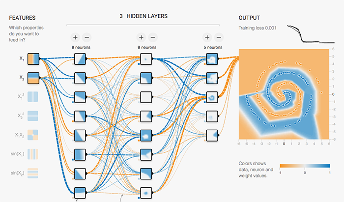
✅ Question 1.9: Now, finally, focus on the dataset with the spiral - the one at the lower right. What is the minimal deep net you can construct that allows you to find a spiral separation boundary? Watch the graph at the upper right - does it appear to be hopping among various local minima?
✎ Put your answers here!
© Copyright 2023, Department of Computational Mathematics, Science and Engineering at Michigan State University.

