Data sets#
These data sets are largely taken from downloads of the ISLR textbook’s R package. A few of them have required some modification to make it a bit easier. I’ve also included some sample data sets generated for various notebooks in the lectures. Notes on each are below. For the data sets generated by Dr. Munch, the code for generation is also included.
Advertising#
TODO: Dataset info
Auto#
TODO: Dataset info
Boston: Do not use#
While I have included this data set in the folder as it is often used in the ISLR and ISLP book, we will not be using it in class. This is due to the major ethical concerns that have resulted in its removal from sklearn.
Carseats#
ChickenEgg#
Dr. Munch generated this data as a simple 2D classification example. The data set has inputs \(x_1\) and \(x_2\), with \(y\) given by Label.
The Bayes classifier is
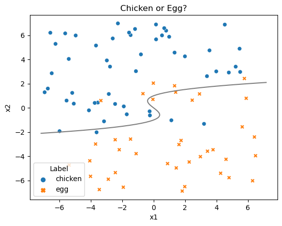
The code used to generate this data is below.
def generateData(N=90,xBounds = [-7,7],yBounds = [-7,7],sigma=1, seed = None):
    # Generating data where the label is determined by being on one side or the
    # other of $y^3-y-x = 0$.
    # Adding noise so it's not cleanly separated
    np.random.seed(seed)
    DataX = np.random.uniform(xBounds[0],xBounds[1],[N,1])
    DataY = np.random.uniform(yBounds[0],yBounds[1],[N,1])

    Data = np.concatenate([DataX,DataY], axis = 1)
    Noise = np.random.normal(0, sigma, N)
    Check = Data[:,1]**3 - 4*Data[:,1] - (Data[:,0]+Noise)
    def ChickOrEgg(z):
        if z>0:
            return 'chicken'
        else:
            return 'egg'
    Label = [ChickOrEgg(z) for z in Check]


    Data = pd.DataFrame(Data, columns = ['x1','x2'])
    Data['Label'] = Label

    return Data


# Generate the data
Data = generateData(N = 90, seed = 48824)

# Plot the figure
sns.scatterplot(data = Data, x = 'x1', y = 'x2', hue = 'Label', style = 'Label').set(title = 'Chicken or Egg?')
ty = np.linspace(-2.1,2.1,100)
tx = ty**3 - ty
plt.plot(tx,ty, color = 'grey')
Clustering example data#
Clustering-ToyData#
Dr. Munch made these data sets for use in the example hierarchical clustering module.
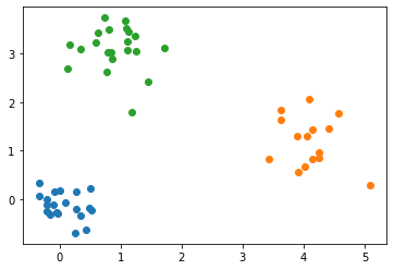
np.random.seed(1)
n1 = 20
X1 = np.random.normal((0,0), .3, (n1,2))

n2 = 15
X2 = np.random.normal((4,1), .5, (n2,2))

n3 = 21
X3 = np.random.normal((1,3), .6, (n3,2))


for A in [X1,X2,X3]:
    plt.scatter(A[:,0],A[:,1])

X = np.concatenate([X1,X2,X3],axis = 0)
np.random.shuffle(X)
Clustering-ToyData2#
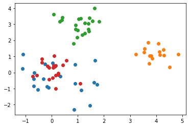
np.random.seed(1)
n1 = 20
X1 = np.random.normal((0,0), 1, (n1,2))
n1b = 20
X1b = np.random.normal((0,0), 0.5, (n1b,2))

n2 = 15
X2 = np.random.normal((4,1), .7, (n2,2))

n3 = 21
X3 = np.random.normal((1,3), .5, (n3,2))


for A in [X1,X2,X3,X1b]:
    plt.scatter(A[:,0],A[:,1])

X = np.concatenate([X1,X2,X3,X1b],axis = 0)
np.random.shuffle(X)
College#
TODO: Dataset info
Credit#
TODO: Dataset info
Default#
Deep learning examples#
DL-toy-data#
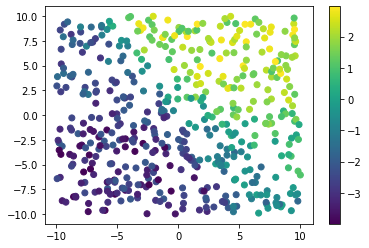
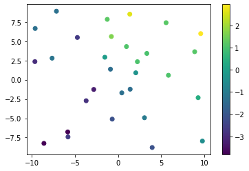 Code used for some example creations in the deep learning module. Dr. Munch generated this using the following code:
w = np.array([(1,2,1),(-1,0,1),(3,-1,-1)]) #<----- Original choices
beta = np.array((-1,2,1,-2))               #<----- of matrices

np.random.seed(0)
X = np.random.random((30,2))*20-10
y = []
for i in range(30):
    y.append(MyFirstNN(X[i,0],X[i,1],w, beta))
y = np.array(y)

ynoise = y + np.random.random(30)*2-1

data = np.concatenate((X,ynoise.reshape(-1,1)),axis = 1)
DL-toy-data-bigger#
def MyFirstNN(X1,X2,w, beta):

    X = np.array((X1,X2))
    A = []

    for i in range(3):
        Ai = w[i,0] + np.dot(w[i,1:],X)
        Ai = 1/(1+np.exp(-Ai))
        A.append(Ai)

    A = np.array(A)

    Y = beta[0] + np.dot(beta[1:], A)

    return Y


w = np.array([(1,2,1),(-1,0,1),(3,-1,-1)]) #<----- Original choices
beta = np.array((-1,2,1,-2))               #<----- of matrices

np.random.seed(0)
n= 500
X = np.random.random((n,2))*20-10
y = []
for i in range(n):
    y.append(MyFirstNN(X[i,0],X[i,1],w, beta))
y = np.array(y)

ynoise = y + np.random.random(n)*2-1

data = np.concatenate((X,ynoise.reshape(-1,1)),axis = 1)
DL-ToyImage#
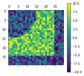
An image used to try out convolutional filters in the CNN module. Data generated using the following code:
np.random.seed(48824)
M = np.random.random((30,30))
M = np.round(10*M, 1)
for i in range(30):
    for j in range(30):
        if i**2 + j**2 < 15**2:
            M[i,j] -= 10

M[25:,:] -=10
M[:25,25:]-=10
Hitters#
Note that this version is slightly different than versions that can be found online. As far as I can tell, it’s just that this particular file has the player names in an entry column.
OJ#
Polynomial toy data set#
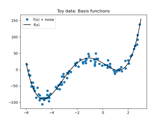
Generated to be useful for the Chapter 7 stuff on polynomial regression, step functions, and splines.
# Set the random seed for reproducibility
np.random.seed(42)

# Define the polynomial
f = lambda x: (x+2)*(x-2)*(x+6)*x+20

# Generate data
x_data = np.random.uniform(-6, 3, 100)
y_data = f(x_data) + np.random.normal(0, 10, size=x_data.shape)

# Generate data for plotting
x_plot = np.linspace(-6, 3, 100)
y_plot = f(x_plot)

# Create a DataFrame to store the data
toy_data = pd.DataFrame({'x': x_data, 'y': y_data})

plt.plot(x_data,y_data, 'o', label = 'f(x) + noise')
plt.plot(x_plot, y_plot, 'k', label = 'f(x)')
plt.legend()
plt.title('Toy data: Basis functions')
Portfolio#
Portfolio2#
TODO: Dataset info
Smarket#
TODO: Dataset info
SVM Examples#
Synthetic data generated by Dr. Munch for the SVM labs.
SVM-Data#
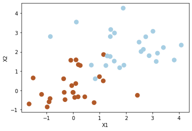
# Generating random data: 20 observations of 2 features and divide into two classes.

np.random.seed(5)
n = 50
X = np.random.randn(n,2)
y = np.repeat([1,-1], n/2)
X[y == -1] = X[y == -1]+2

data = np.concatenate((X,y.reshape(-1,1)), axis = 1)
np.random.shuffle(data)
SVM-Data2#
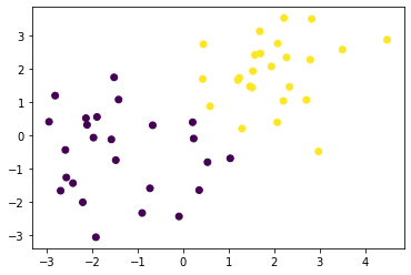
# Generating random data: 50 observations of 2 features and divide into two classes.
# This one is more spread about than original
np.random.seed(48824)
n = 50
X = np.random.randn(n,2)
y = np.repeat([1,-1], n/2) #
X[y == -1] = X[y == -1]+2
X[y == 1] = X[y == 1]-1.5
X[:,1][y == 1] = X[:,1][y == 1]+.9
y = y*-1

data = np.concatenate((X,y.reshape(-1,1)), axis = 1)
np.random.shuffle(data)
SVM-Data3#
Generated to emphasize usefulness of kernel options in SVM.
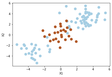
np.random.seed(8)
n = 100
k = int(n/4)
X = np.random.randn(n,2)
X[:2*k] = X[:2*k] +3
X[2*k+1:3*k] = X[2*k+1:3*k] -3
y = np.concatenate([np.repeat(-1, 3*k), np.repeat(1,n-3*k)])
data = np.concatenate((X,y.reshape(-1,1)), axis = 1)
Wage#
Weekly#
TODO: Dataset info
