In order to successfully complete this assignment, you must follow all the instructions in this notebook and upload your edited ipynb file to D2L with your answers on or before 11:59pm on Friday March 26th.
BIG HINT: Read the entire homework before starting.
Homework 4: Practice Quizes
In this homework, we will exploring four different examples of in-class quizzes students had in previous semesters of this course. These problems are intended to give student's exposure to the style of questions asked on quizzes and help you practice. Please finish the entire Jupyter Notebook and turn in your edited file using the MSU D2L Website.
Your instructors recommend doing one question at a time. Set a timer for 20-30 minutes and see how much of the question you can answer. We hope this will get you used to getting a timed quiz complete during class.
Outline for Homework 1
Recall that on the first day of class we showed how computers can represent different colors as vectors. Specifically we have a 3-vector $[R,G,B]$ that stores the amount of red, green, and blue that appears in a specific pixel. In that notebook we took the entries to be floats in the range of 0-1. Today we will again be working with RGB color vectors, but in this quiz the values of the entries will be integers in the range of 0-255.
Recently in class we have discussed how to use matrix multiplication to apply affine transformations to a set of points in a picture. In this quiz we will be applying transformations to the color vectors associated to each pixel in the image.
%matplotlib inline
import matplotlib.pylab as plt
import numpy as np
import sympy as sym
sym.init_printing()
The following code will download and display an image from the given url.
import imageio

#from urllib.request import urlopen, urlretrieve
#from scipy.misc import imsave

url = 'http://www.ideachampions.com/weblogs/iStock_000022162723_Small.jpg'
#url = 'http://colortutorial.design/rgb.jpg'
im = imageio.imread(url)
plt.imshow(im)

The functions below will convert between images represented by 3-dimensional arrays of shape $(h,w,3)$, and numpy matrices of size $3 \times n$. In the $3 \times n$ matrix each column represents the color of an individual pixel of our image.
def image2matrix(image):
    '''Turns an image into a numpy matrix of size 3 x (h*w).'''
    h,w,_ = image.shape
    return np.matrix(image.reshape(h*w,3)).T

def matrix2image(matrix,h,w):
    '''Turns a 3xn matrix into a numpy array of shape (h,w,3).'''

    if h*w != matrix.shape[1]:
        raise Exception("Matrix must have length of h*w!")

    return np.array(matrix.T).reshape(h,w,3).astype(int).clip(0,255)
Below is the image matrix that we will be using for Question 1. It is saved as im_mat.
h,w,_ = im.shape
im_mat = image2matrix(im)
im_mat.shape
If we apply an affine transformation to im_mat we are changing the color vectors associated to the pixel.
The idea is that if we have a matrix $M$ and a color vector $x = (R,G,B)^T$, then $Mx$ will be a new $ 3 \times 1$ matrix that represents a new color.
sepia = np.matrix('0.393,0.769,0.189;0.349,0.686,0.168;0.272,0.534,0.131')
sepia_mat = sepia * im_mat
plt.imshow(matrix2image(sepia_mat,h,w))

✅ QUESTION 1: (5pts) Apply the following grayscale transformation below to the image matrix im_mat. Save the result as new_image_matrix.
## Edit this cell for your work.
grayscale = np.matrix(np.ones([3,3]))/3

#new_image_matrix =
from answercheck import checkanswer

# we suppress the output and only check 100 values of your matrix to speed things up.
checkanswer.detailedwarnings = False
checkanswer.matrix(new_image_matrix[:,1000:1100],"c0c5f50c51db1b7a528b6fdd7425cac8");
The code below will display your edited image.
plt.imshow(matrix2image(new_image_matrix,h,w))
✅ QUESTION 2: (5pts) Find the determinant of the sepia and grayscale matrices. Save your ansers as det_sepia and det_gray, respectively.
##Work in this cell
sepia = np.matrix('0.393,0.769,0.189;0.349,0.686,0.168;0.272,0.534,0.131')
grayscale = np.matrix(np.ones([3,3]))/3

#det_sepia =
#det_gray =
from answercheck import checkanswer
checkanswer.detailedwarnings = True
checkanswer((det_sepia,det_gray),"924c2a9fa81245883d7bce7547ae91f0");
✅ QUESTION 3: Explain why the sepia transformation is reversible, but it is not possible to reverse the grayscale transformation provided above.
YOUR ANSWER HERE
In the last two questions we ask that you produce transformations that have a specific affect on the provided color vectors.
✅ QUESTION 4: (5pts) Create a $3 \times 3$ matrix A that swaps the red and blue values in a color vector.
That is we want A to be a matrix such that $Ax = x'$ where $x = [R,G,B]^T$ and $x' = [B,G,R]^T$.
Hint. Think about elementary row operations.
## Edit the entries below to make the appropriate matrix.
A = np.matrix([[0,0,0],[0,0,0],[0,0,0]])

#You don't need to edit the following line
sym.Matrix(A)
from answercheck import checkanswer
checkanswer.matrix(A,"2c2d2e407389eabeb6d90894565c830f")
The following code will display the color-swapped image.
plt.imshow(matrix2image(A*im_mat,h,w))

The formula for producing the negative of an image is given by
$$ R_{\text{neg}} = 255-R,\\ G_{\text{neg}} = 255-G, \\ B_{\text{neg}} = 255-B.$$Translating these transformations into a matrix equation gives rise to the following:
$$ \left[ \begin{matrix} R_{\text{neg}} \\ G_{\text{neg}} \\ B_{\text{neg}} \end{matrix} \right] = \left[ \begin{matrix} -1 & 0 & 0\\ 0 & -1 & 0\\ 0 & 0 & -1 \end{matrix} \right] \left[ \begin{matrix} R \\ G \\ B \\ \end{matrix} \right] + \left[\begin{matrix} 255\\ 255 \\ 255 \end{matrix} \right] $$✅ QUESTION 5: (5pts)
Create an equivalent $3 \times 4$ matrix B such that $Bx = x_{\text{neg}}$ where $$ x =\begin{bmatrix} R \\ G\\ B \\ 1 \end{bmatrix},\, \text{and} \,x_{\text{neg}} = \begin{bmatrix} R_{\text{neg}}\\ G_{\text{neg}} \\ B_{\text{neg}} \end{bmatrix}$$
Hint. Remember the fractal section.
## Edit the entries below to make the appropriate matrix.
B = np.matrix([[0,0,0,0],[0,0,0,0],[0,0,0,0]])

#You don't need to edit the following line
sym.Matrix(B)
from answercheck import checkanswer
checkanswer.matrix(B,"6df638d913b745cf0369556cdc7e83c2")
2. Recurrence Relations

In this question we will introduce and solve recurrence relations by using matrices, eigenvalues, and eigenvectors.
A sequence $(a_n)_{n=0}^\infty$ is an infinite list of numbers $(a_0, a_1, a_2, a_3, \dots)$. In this class we can think about them as being infinite length vectors. One way to describe a sequence is to give an iterative rule that defines the next entry of the sequence in terms of previous ones. This is called a recurrence relation.
For example, one of the most famous sequences of numbers is the Fibonacci sequence. This sequence goes as follows $$(0, 1, 1, 2, 3, 5, 8, 13, 21, 34, 55, 89, 144, 233, 377,\dots)$$
Instead of having to write out the infinite list of numbers we can just describe a rule to generate the next element in the sequence. For the Fibonacci sequence the rule is defined by the relation $$f_n = f_{n-1} + f_{n-2}.$$ That is to calculate the next entry in the sequence you add the previous two. Now there are many sequences of numbers that satisfy this rule, so to specify the Fibonacci sequence we also need to specify the start of the sequence. Specifically, that $f_0=0, \,f_1=1.$
We can use matrices to encode recurrence relations and compute future values by using matrix multiplication. For the Fibonacci sequence it looks like the following. Let $$v_n := \begin{pmatrix} f_n \\ f_{n-1} \end{pmatrix}, \, \text{ and } A = \begin{pmatrix} 1 & 1 \\ 1 & 0 \end{pmatrix}.$$ Then we notice that $v_n = Av_{n-1}$ or more generally, we have that $A^{n-1}v_1 = v_n$. Specifically,
$$Av_{n-1}= \begin{pmatrix} 1 & 1 \\ 1 & 0 \end{pmatrix} \begin{pmatrix} f_{n-1} \\ f_{n-2} \end{pmatrix} = \begin{pmatrix} f_{n-1}+f_{n-2} \\ f_{n-1} \end{pmatrix} = \begin{pmatrix} f_n \\ f_{n-1} \end{pmatrix} = v_n $$For a specific example notice that for the Fibonacci sequence we have $v_5 = (5,3)^T$, $v_6 = (8,5)^T$, and that $v_6 = A v_5 = A^5v_1$.
Matrix multiplication is one way of computing these values but it has the drawback that to find the 100th entry in the sequence you need to also compute the first 99 entries as well.
Luckily for us the collection of solutions to a given recurrence relation forms a vector space and we will use this structure to write a formula for a general solution in terms of the eigenbasis.
%matplotlib inline
import matplotlib.pylab as plt
import numpy as np
import sympy as sym
sym.init_printing()
✅ QUESTION 1: (5pts) Find a matrix $B$ that represents the recurrence relation $$b_n = 5b_{n-1} - 4b_{n-2}$$
Hint. Define $v_n = (b_n,b_{n-1})^T$. Your matrix should be $2 \times 2$ and satisfies the equation $Bv_{n-1} = v_{n}$.
## Edit this cell for your work.
#B =
from answercheck import checkanswer
checkanswer.detailedwarnings = False
checkanswer.matrix(B,"496f5b1ff53292b14df4589781a8d5c3");
✅ QUESTION 2: (5pts) Compute $b_{10}$ for the recurrence relation $b_n = 5b_{n-1} - 4b_{n-2}$ when $b_1 = 4, b_0=2.$ Save your value as b10 for answercheck.
##Do your work here
# b10 =
from answercheck import checkanswer
checkanswer.detailedwarnings = False
checkanswer.float(b10,"56b48e42a1b4913229ef0c1c39ca7cc4");
In the next three questions we will discuss how to use vectorspaces to give a direct formula for computing sequences that satisfy a particular recurrence relation.
In the next questions we will try to find a basis for the sequences that satisfy the recurrence relation given by $a_n = 2a_{n-1} + a_{n-2} -2a_{n-3}.$
This rule can be encoded using the matrix $$A = \begin{bmatrix} 2 & 1 & -2 \\ 1 & 0 & 0 \\ 0 & 1 & 0 \end{bmatrix}$$
✅ QUESTION 3: (5pts) Find the eigenvalues and eigenvectors of the matrix $A.$ Save the eigenvalues as lambda1, lambda2, and lambda3 in increasing order so $\lambda_1 < \lambda_2 < \lambda_3$. Save the eigenvector associated to the largest eigenvalue as e_vect.
## put work here


# lambda1 =
# lambda2 =
# lambda3 =
# e_vect =
from answercheck import checkanswer
checkanswer.detailedwarnings = False
checkanswer.vector([lambda1,lambda2,lambda3],"5b45740e77f757e93909c339151989c9");
from answercheck import checkanswer
checkanswer.detailedwarnings = False
checkanswer.eq_vector(e_vect,"443e6b36745607a9900c90882d5eb805");
Now notice that for any eigenvalue $\lambda$ of $A$ with associated eigenvector $v$, we have that $$ v = c \begin{bmatrix} \lambda^2 \\ \lambda \\ 1 \end{bmatrix}.$$
That is to say if we rescale our vector e_vect by a factor of 1/e_vect[-1] we get the vector $[\lambda_3^2,\lambda_3,1]^T$. This is important for the next question!
w = e_vect/e_vect[-1]
sym.Matrix(w)
So far we have only looked at the matrix $A$ encoding the recurrence rule $a_n = 2a_{n-1} + a_{n-2} -2a_{n-3}.$ In order to find a sequence we need to specify our 3 initial values $a_0, a_1,$ and $a_2.$
Then like before we can compute $a_3$ as the first entry in the vector $v_3$ by the matrix multiplication $Av_2 = v_3$, where $v_n = [a_n,a_{n-1},a_{n-2}]^T.$
✅ QUESTION 4: (5pts) Let $\lambda$ be an eigenvalue for the matrix $A$. Use the terms "eigenvalue" and "eigenvector" to explain why taking $a_2 = \lambda^2,\, a_1 = \lambda, \,a_0 = 1 $ yields $a_3 = \lambda^3$.
YOUR ANSWER HERE
Following the explanation that is the answer to the previous question, it is easy to show that $a_n = \lambda^n$ for all $n \geq 0$!
A fact that is harder to show, but still true, is when the eigenvalues are all distinct (like in our case) these sequences form a vector space basis for all solutions to the recurrence relation $a_n = 2a_{n-1} + a_{n-2} -2a_{n-3}.$
That is to say that all solutions to our recurrence relation are linear combinations of the three sequences, $(\lambda_1^n)_{n=0}^\infty, (\lambda_2^n)_{n=0}^\infty, (\lambda_3^n)_{n=0}^\infty.$ Therefore for any sequence $(a_n)_{n=0}^\infty$ that satisfies the recurrence relation there exists constants $c_1,c_2,$ and $c_3$ such that
$$ a_n = c_1 \lambda_1 ^n + c_2 \lambda_2^n + c_3 \lambda_3^n,$$for all $n \geq 0!$
This means that if we are given inital values of $a_0,a_1,$ and $a_2.$ The values of $c_1,c_2,c_3$ are just the coordinates for the vector $[a_2,a_1,a_0]^T$ in the basis given by the vectors $\{[\lambda_1^2,\lambda_1,1]^T,[\lambda_2^2,\lambda_2,1]^T,[\lambda_3^2,\lambda_3,1]^T\}$.
In the next question we will find the values for the coefficients when $a_2 = 4, a_1 = 2, a_0 = 2.$
Let $\lambda_1,\lambda_2, \lambda_3$ be the eigenvalues for $A$ given in increasing order. You found these values in Question 2.
✅ QUESTION 5: (5pts) Express the vector $v_2 = \begin{bmatrix} 4 \\ 2 \\ 2 \end{bmatrix}$ in terms of the basis $\{w_1,w_2,w_3\}$, where $w_i = [\lambda_i^2,\lambda_i,1]^T$. Save your new vector as c.
##Show your work here
w1 = np.matrix([lambda1**2,lambda1,1]).T
w2 = np.matrix([lambda2**2,lambda2,1]).T
w3 = np.matrix([lambda3**2,lambda3,1]).T
v2 = np.matrix("4;2;2")

#c =
from answercheck import checkanswer

checkanswer.vector(c,"9afaa124239d033a645d277f7c8ad41a");
Now using the formula we see that it is easy to compute arbitrary elements of the sequence.
##Either code will directly compute the 10th value of sequence.

#a10 = c[0]*lambda1**10+c[1]*lambda2**10+c[2]*lambda3**10
a10 = np.dot( np.power([lambda1,lambda2,lambda3],10) ,c)
a10
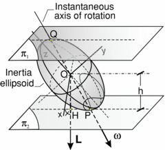
The machinery of developing eigenvectors and eigenvalues was originally done to explain rotational dynamics. You might be familiar with some of the equations for rotation in the plane such as
where L is the angular momentum, I is the moment of inertia, and $\omega$ is the angular velocity. It turns out the same equation holds in 3-dimensional rotation, and this becomes a matrix equation. $I$ will now be given as a 3x3 matrix, and $\omega$ and $L$ represent vectors. The principal axes of rotation are those directions where $L$ is in the same direction as $\omega$, where $$I \omega = L = \lambda \omega,$$ so finding the principal axes is an eigenvalue problem. The values of $\lambda$ represent the moment of inertia about the corresponding axis.
Take the moment of inertia matrix $I$ for a 3D ridged body given by $$I=\begin{bmatrix} 7 & 4 & 5 \\ 4 & 10 & 2 \\ 5 & 2 & 8 \end{bmatrix}$$
%matplotlib inline
import matplotlib.pylab as plt
import numpy as np
import sympy as sym
sym.init_printing()
✅ QUESTION 1: (2 pts) Define a Numpy matrix $A$ to be the moment of inertia matrix above (We don't want to call it $I$ since that is usually reserved for the identity matrix).
# Put your answer to the above question here
from answercheck import checkanswer
checkanswer.matrix(A,"1edd5b825b5c67ebdb15a8f0b276a927");
✅ QUESTION 2: (5 pts) Find the eigenvalues and eigenvectors of the moment of inertia matrix.
Save the eigenvalues as lambda1, lambda2, and lambda3 in increasing order so lambda1 <lambda2 < lambda3.
# Put your answer to the above question here
from answercheck import checkanswer
checkanswer.detailedwarnings = False
checkanswer.vector([lambda1,lambda2,lambda2],'228139b44f7ef63d552eaf20458929bb')
The major axis is the axis which corresponds to the eigenvector with the largest eigenvalue. Save the major axis in a variable called m_axis.
# Put your answer to the above question here
from answercheck import checkanswer
checkanswer.detailedwarnings = False
checkanswer.eq_vector(m_axis,'34e96454efdb65f22d06cda5d6d28781')
✅ QUESTION 3: (2 pts) Verify that the eigenvectors are linearly independent by calculating the rank of an appropriate matrix.
# YOUR CODE HERE
raise NotImplementedError()
✅ QUESTION 4: (2 pts) Next, verify the eigenvectors are linearly independent by calculating a determinant.
# YOUR CODE HERE
raise NotImplementedError()
✅ QUESTION 5:(5 pts) Explain how the calculation of this determinant shows the vectors are linearly independent.
YOUR ANSWER HERE
✅ QUESTION 6: (5 pts) Take the vector $b=[2,2,2]$. Write this vector as a linear combination of the eigenvectors. (For the answer, just write the coefficients as a vector)
#Put answer here.
from answercheck import checkanswer
checkanswer.detailedwarnings = False
checkanswer.eq_vector(x,"59c224734374df4a3747c77e0976fbfb");
✅ QUESTION 7: (5 pts) Do the eigenvectors constitute a basis for $\mathbb{R}^3$? Why or why not?
YOUR ANSWER HERE
4. Reverse Transforms

With the transformations we have worked on before, we were given a transformation, and we determined what was the end result of transformation for a given set of points. We will look at the opposite problem, where we are given the end result, and we need to find out where the points came from. This transformation will be given as the matrix inverse.
%matplotlib inline
import matplotlib.pylab as plt
import numpy as np
import sympy as sym
sym.init_printing()
Part I
For coordinates in 2 dimentions of the form $x = \left[ \begin{matrix} x\\ y\\ 1 \end{matrix} \right]$, translation of 3 units to the right and 5 units up can be given by the equation $Ax=b$ using the following ($ 3 \times 3$) Matrix $A$:
A = np.matrix([[1,0,3], [0,1,5],[0,0,1]])
sym.Matrix(A)
✅ QUESTION 1.a: (3pts) Describe in words the action of the inverse operation, that is, how given a point $b = \left[ \begin{matrix} b_1\\ b_2\\ 1 \end{matrix}\right]$, how can you get back to x?
YOUR ANSWER HERE
✅ QUESTION 1.b: (3pts) Write down the inverse matrix $A^{-1}$ as another translation matrix (Store this as a numpy matrix named A_inv)
#Put your answer to the above quesiton here.
from answercheck import checkanswer
checkanswer.matrix(A_inv,"005427e8ac656450ae1ddb6a19a87b68");
✅ QUESTION 1.c: (2pt) Verify through matrix multiplication that $AA^{-1} = I$, the identity matrix.
# YOUR CODE HERE
raise NotImplementedError()
Part 2
A matrix which rotates 2D points counterclockwise through an angle $\theta$ is given by the following matrix:
$$ \left[ \begin{matrix} \cos{\theta} & -\sin{\theta} \\ \sin{\theta} & \cos{\theta} \end{matrix} \right] $$✅ QUESTION 2.a: (3pts) Let $\theta = 2\pi/3$ radians (120 degrees). Give the matrix (call it R) for rotating counterclockwise 120 degrees.
#Put your answer to the above question here
from answercheck import checkanswer
checkanswer.matrix(R,"9c3f5e8dd4b77ea1d98ef98ba0c0b974");
✅ QUESTION 2.b: (2pts) Perform the matrix multiplication $R \times R \times R$. Save your answer in a variable R3.
# YOUR CODE HERE
raise NotImplementedError()
R*R*R
✅ QUESTION 2.c: (3pts) In. your own words, explain the answer from question 2.b.
YOUR ANSWER HERE
Part III
One of the elementary matrix operations we have used is the switching of rows. If we switch the rows corresponding to x and y, geometrically, this corresponds to a reflection about the axis y = x.
✅ QUESTION 3.a: (3pts) Write down the matrix which switches the first two rows of a 3 x 3 matrix (call it S).
#Put your answer to the above question here.
from answercheck import checkanswer
checkanswer.matrix(S,"769c14b030a58dd867fa2aece33520ef");
✅ QUESTION 3.b: (3pts) What is the inverse of S?
YOUR ANSWER HERE
✅ QUESTION 3.c: (3pts) Explain why the inverse of S is what it is.
YOUR ANSWER HERE
Congratulations, we're done!
Turn in your assignment using D2L no later than 11:59pm on the day of class. See links at the end of this document for access to the class timeline for your section.
Written by Drs. Matthew Mills and Rongrong Wang, Michigan State University

This work is licensed under a Creative Commons Attribution-NonCommercial 4.0 International License.