In order to successfully complete this assignment, you must follow all the instructions in this notebook and upload your edited ipynb file to D2L with your answers on or before 11:59pm on Friday October 23rd.
BIG HINT: Read the entire homework before starting.
**_WARNING:_** Many of the matrixes used in this homework are very big. Be caareful displaying these matrices using the sym.Matrix. This may cause some of your web browsers to have a difficult time rendering all of the latex.
Download New Answer Check Program
This homework takes advantage of a new answercheck. ALthough you can still use the old one, the new one will make the output much cleaner and easier to read. Download the new answercheck using the following cell
from urllib.request import urlretrieve

urlretrieve('https://raw.githubusercontent.com/colbrydi/jupytercheck/master/answercheck.py',
            'answercheck.py');
Homework III: Network Vulnerability
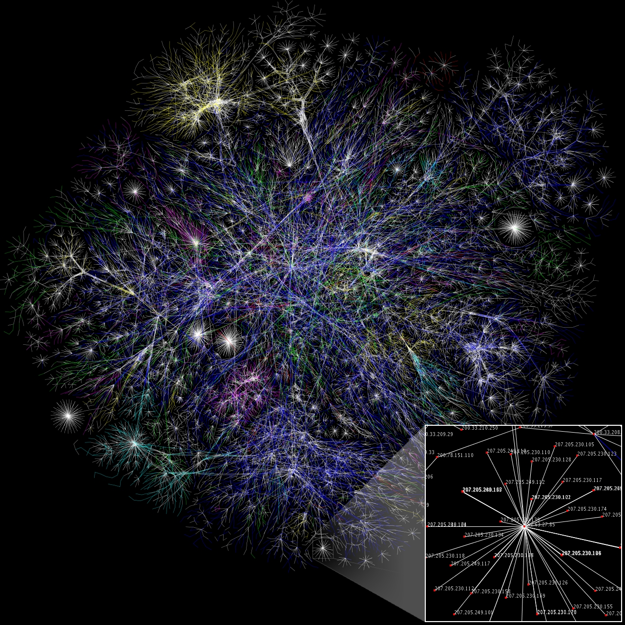
Image from: https://en.wikipedia.org/wiki/Internet_Mapping_Project
By simply observing a graph such as the above, it can be hard to intuit anything meaningful. But graphs and networks are turning up at the frontiers of fields as diverse as Data Science, Quantum Information & Computing, and Chaos & Complexity Theory. In this assignment we will look at Internet networks. For fun, watch the following video. This is not required but your instructor really liked this video when they were learning about how networks work (yes it is an old video):
from IPython.display import YouTubeVideo
YouTubeVideo("PBWhzz_Gn10",width=640,height=360, cc_load_policy=True)
Some of us conducting research on, and related to, these networks are finding seemingly magical information hidden in the eigenvalues and eigenvectors of matrix representations of these graphs. For instance, we may quantify the vulnerability of a computer network to a random outage using only the second smallest eigenvalue, $\lambda_{2}$, of the normalized graph Laplacian of the network.
The study of graphs and their relationships to eigenvectors / eigenvalues is known as Spectral Graph Theory.
# Here are some libraries you may need to use
%matplotlib inline
import numpy as np
import sympy as sym
import networkx as nx
import matplotlib.pyplot as plt
sym.init_printing(use_unicode=True)
Basic Graph Theory: Jargon Ahead
Consider the following extremely quick video introducing the concept of graphs:
from IPython.display import YouTubeVideo
YouTubeVideo("m-KUiibR4Xs",width=640,height=360, mute=0)
The graph
A graph, $G$, is a mathematical object that may be described by a tuple $G=(V,E)$, where $V=\{v_1,v_2,\ldots ,v_n\}$ are the vertices, or nodes, and $E=\{(u,v):u,v\in V\}$ is the set of edges connecting the vertices. Note that we typically do not allow $(v,v)$ to be in $E$; this represents a self-loop, or edge.
The adjacency matrix
In this course we will represent the graph with an adjacency matrix, usually denoted $A$. The adjacency matrix, $A$, of a graph, $G$, is a matrix of $1$s and zeros, where
$$A_{ij} = 1$$if $(i,j)\in E$, and
$$A_{ij} = 0$$otherwise.
Consider the following graph. Think about how you would represent this graph as a matrix in Python. For this homework think about the nodes of the graphs as power consumers (i.e., dinosaur fences) and the edges of the graph powerlines supplying power to the nodes.

Image from: http://www.algolist.net/
</a>Here is the same graph depicted above encoded as an adjacency matrix in numpy:
%matplotlib inline
import numpy as np

import sympy as sym
sym.init_printing(use_unicode=True)

A = np.array([[0,0,0,1,0],[0,0,0,1,1],[0,0,0,0,1],[1,1,0,0,1],[0,1,1,1,0]])

sym.Matrix(A)
Now we can use the networkx to draw the graph:
import networkx as nx
import warnings
warnings.filterwarnings("ignore", category=UserWarning)

G = nx.Graph(A)
pos=nx.spring_layout(G)
nx.draw_networkx_nodes(G,pos)
nx.draw_networkx_edges(G,pos)
plt.axis('off')
plt.show()

Notice that the location of the nodes is not specified in the graph description, so make sure you can see that the graph depicted in the code is the same as the graph shown in the example above.
The graph Laplacian matrix
We may, alternatively, represent a graph by its graph Laplacian, sometimes also called the admittance matrix (Cvetković et al. 1998, Babić et al. 2002) or Kirchhoff matrix,
$$L = D-A$$where $A$ is the adjacency matrix and $D$ is a specific diagonal matrix whose entries $D_{ii} = \sum_{j=1}^{n}A_{ij}$ are the number of edges connected to the $i^{th}$ vertex. (You may want to think about this for a minute until it's obvious why we can just sum over the rows of $A$ to get the entries of $D$.)
The following code generates the the matrix D for the above graph.
d = np.sum(A,1) # Make a vector of the sums.
D = d*np.identity(5) #Multiply the vector by Identity matrix to get D
sym.Matrix(D)
Then the Laplacian is can be defined as follows:
L = D-A
sym.Matrix(L)
The normalized graph Laplacian matrix
We may also represent a graph by its normalized graph Laplacian,
$$\begin{align*} N &= D^{-\frac{1}{2}}(D-A)D^{-\frac{1}{2}} \\ &= D^{-\frac{1}{2}}LD^{-\frac{1}{2}} \end{align*}$$where $A$ and $D$ are as above and $D^{\frac{1}{2}}$ (i.e. the square root of a matrix) extends the notion of square root from numbers to matrices. A matrix $D^{\frac{1}{2}}$ is said to be a square root of $D$ if the matrix product $D^{\frac{1}{2}}D^{\frac{1}{2}}$ is equal to $D$. The inverse of $D^{\frac{1}{2}}$ is denoted as $D^{-\frac{1}{2}}$ and still defined as $D^{\frac{1}{2}}D^{-\frac{1}{2}} = I$
Since we call $L=D-A$ the graph Laplacian, can you see why we call $N$ normalized?
Part I: The Complete Graph
✅ **DO THIS:** Run the following code to generate a complete graph, $K_{m}$, on $m$ vertices (in this case m=10). Note that for a Complete Graph each vertex is connected to every other vertext, hence the name "complete".
# Simply run this cell.
m = 10 # number of nodes
Km = nx.complete_graph(m) # initialize graph

## draw graph
pos=nx.circular_layout(Km) # positions for all nodes

### nodes
nx.draw_networkx_nodes(Km,pos,
                       node_color='c',
                       node_size=400,
                       alpha=0.8)

### edges
nx.draw_networkx_edges(Km,pos,
                       width=2,alpha=0.5,edge_color='b')

nx.draw_networkx_labels(Km,pos,font_size=12)

plt.axis('off')
plt.show() # display

✅ **DO THIS:** Generate the adjacency matrix, $A_{K_m}$, of the above complete graph, $K_{m}$, and print the result. (Hint: We recommend that you use package, such as the one you imported above: NetworkX)
# adjacency matrix code here
from answercheck import checkanswer
checkanswer.detailedwarnings = False
checkanswer.matrix(AKm,"b8570745b45d7aad75c61a331a96d764");
✅ **DO THIS:** Generate the $D_{K_m}$ and $D_{K_m}^{-1}$ matrices of the above complete graph, $K_{10}$, and show via computation in Python that your matrices are, indeed, inverses of each other.
# D and D_inv matrices' code here
from answercheck import checkanswer
checkanswer.detailedwarnings = False
checkanswer.matrix(D,"9aa12ea770f60f509f7894939e4554b3");
from answercheck import checkanswer
checkanswer.detailedwarnings = False
checkanswer.matrix(D_inv,"ba6a392f4cfe0907cdd4ff2e20fed36a");
✅ **DO THIS:** Calculate the normalized Laplacian $N_{K_{m}}$.
# your code goes here
from answercheck import checkanswer
checkanswer.detailedwarnings = False
checkanswer.matrix(N,"6c607038701e2d0f11a3597eb3e271fa");
✅ **DO THIS:** Using the standard that $0 = \lambda_{1}\leq\lambda_{2}\leq\ldots\leq\lambda_{n}$, generate an ordered list of eigenvalues, $\lambda_{i}$, of the normalized Laplacian $N_{K_{m}}$.
Print the second smallest eigenvalue, $\lambda_{2}$, of this matrix.
# your code goes here
from answercheck import checkanswer
checkanswer.detailedwarnings = False
checkanswer.matrix(eig,"b0cba9a71fc027cf49fa7697f7209fdc");
✅ **Question:** What is the second smallest eigenvalue , $\lambda_{2}$, of this matrix.
YOUR ANSWER HERE
Part II: The Barbell Graph
A barbell network has two major networks (think office buildings) connected by a single chain of nodes between the network.
✅ **DO THIS:** Run the following cell to generate the barbell graph, $B$.
# Simply run this cell.
n = 30 # number of nodes
B = nx.Graph() # initialize graph

## initialize empty edge lists
edge_list_complete_1 = []
edge_list_complete_2 = []
edge_list_path = []

## generate node lists
node_list_complete_1 = np.arange(int(n/3))
node_list_complete_2 = np.arange(int(2*n/3),n)
node_list_path = np.arange(int(n/3)-1,int(2*n/3))

## generate edge sets for barbell graph
for u in node_list_complete_1:
    for v in np.arange(u+1,int(n/3)):
        edge_list_complete_1.append((u,v))

for u in node_list_complete_2:
    for v in np.arange(u+1,n):
        edge_list_complete_2.append((u,v))

for u in node_list_path:
    edge_list_path.append((u,u+1))

# G.remove_edges_from([(3,0),(5,7),(0,7),(3,5)])

## add edges
B.add_edges_from(edge_list_complete_1)
B.add_edges_from(edge_list_complete_2)
B.add_edges_from(edge_list_path)


## draw graph
pos=nx.random_layout(B) # positions for all nodes

### nodes
nx.draw_networkx_nodes(B,pos,
                       nodelist=list(node_list_complete_1),
                       node_color='c',
                       node_size=400,
                       alpha=0.8)
nx.draw_networkx_nodes(B,pos,
                       nodelist=list(node_list_path),
                       node_color='g',
                       node_size=200,
                       alpha=0.8)
nx.draw_networkx_nodes(B,pos,
                       nodelist=list(node_list_complete_2),
                       node_color='b',
                       node_size=400,
                       alpha=0.8)


### edges
nx.draw_networkx_edges(B,pos,
                       edgelist=edge_list_complete_1,
                       width=2,alpha=0.5,edge_color='c')
nx.draw_networkx_edges(B,pos,
                       edgelist=edge_list_path,
                       width=3,alpha=0.5,edge_color='g')
nx.draw_networkx_edges(B,pos,
                       edgelist=edge_list_complete_2,
                       width=2,alpha=0.5,edge_color='b')

nx.draw_networkx_labels(B,pos,font_size=12)

plt.axis('off')
plt.show() # display

This graph looks like a mess. Let's clean it up by running the following cell which uses a different algorithm to layout the nodes (spring vs. random and circular).
## draw graph
pos=nx.spring_layout(B) # positions for all nodes

### nodes
nx.draw_networkx_nodes(B,pos,
                       nodelist=list(node_list_complete_1),
                       node_color='c',
                       node_size=400,
                       alpha=0.8)
nx.draw_networkx_nodes(B,pos,
                       nodelist=list(node_list_path),
                       node_color='g',
                       node_size=200,
                       alpha=0.8)
nx.draw_networkx_nodes(B,pos,
                       nodelist=list(node_list_complete_2),
                       node_color='b',
                       node_size=400,
                       alpha=0.8)


### edges
nx.draw_networkx_edges(B,pos,
                       edgelist=edge_list_complete_1,
                       width=2,alpha=0.5,edge_color='c')
nx.draw_networkx_edges(B,pos,
                       edgelist=edge_list_path,
                       width=3,alpha=0.5,edge_color='g')
nx.draw_networkx_edges(B,pos,
                       edgelist=edge_list_complete_2,
                       width=2,alpha=0.5,edge_color='b')


plt.axis('off')
plt.show() # display

This is certainly better! We can see that we have two blobs connected by a long path. In fact, those blobs are individual complete graphs connected by a path. If we consider this as a network of two different buildings, just looking at it, we might conclude that this network is far more vulnerable to a random outage (removal of an edge) than the complete graph, $K_{m}$ above. Let's see if $\lambda_{2}$ of this graph's normalized graph Laplacian says anything to this effect.
✅ **DO THIS:** Generate the adjacency matrix, $A_{B}$, of the above barbell graph, $B$, and print the result. (Hint: You may want to use a package, such as the one you imported above: NetworkX)
# adjacency matrix code here
from answercheck import checkanswer
checkanswer.detailedwarnings = False
checkanswer.matrix(A,"6c3e06b733035ca7134fab7036b1a6a1");
A fun way to view such a large adjacency matrix is to use the imshow function
plt.imshow(A)

✅ **DO THIS:** Generate the $D_{B}$ and $D_{B}^{-1}$ matrices of the above barbell graph network, $B$, and show via computation in Python that your matrices are, indeed, inverses of each other.
# D and D_inv matrices' code here
from answercheck import checkanswer
checkanswer.detailedwarnings = False
checkanswer.matrix(D,"a4c62234cd71d11ffef79202af3d9cca");
from answercheck import checkanswer
checkanswer.detailedwarnings = False
checkanswer.matrix(D_inv,"de6dcc4062b82d2a4d992e0f80451926");
✅ **DO THIS:** Calculate the normalized Laplacian $N_{K_{m}}$.
# your code goes here
from answercheck import checkanswer
checkanswer.detailedwarnings = False
checkanswer.matrix(N,"944e3071214ffb8b1eaf88178f02cb11");
✅ **DO THIS:** Using the standard that $0 = \lambda_{1}\leq\lambda_{2}\leq\ldots\leq\lambda_{n}$, compute the eigenvalues, $\lambda_{i}$, of the normalized Laplacian $N_{K_{m}}$.
# your code goes here
from answercheck import checkanswer
checkanswer.detailedwarnings = False
checkanswer.matrix(eig,"2ba29da3bef05fed0a3efb8592498e57");
✅ **DO THIS:** Compare the second smallest eigenvalue, $\lambda_{2}$, of the normalized graph Laplacian of $B$ with thaa of $K_{m}$. Which is smaller?
# YOUR CODE HERE
raise NotImplementedError()
Part III: Your Computer Network
✅ **DO THIS:** Using the code in the following cells, generate your own graph, $Y$, using one of the graph generators here. Pay attention to the parameters that are needed as they can vary between generators. (Note: pos=nx.spectral_layout(Y) will plot your graph using the $2^{nd}$ and $3^{rd}$ eigenvectors as coordinates--cool!)
# Simply run this cell.
n = 60 # number of nodes
# YOUR CODE HERE
raise NotImplementedError()
## draw graph
pos=nx.spring_layout(Y) # positions for all nodes--you may play with this too using spectral_layout(Y), for instance

nx.draw(Y,pos)

plt.axis('off')
✅ **DO THIS:** Describe your graph, $Y$, in words.
YOUR ANSWER HERE
✅ **DO THIS:** Generate the adjacency matrix, $A_{Y}$, of your graph, $Y$, and show the result as an image.
# YOUR CODE HERE
raise NotImplementedError()
✅ **DO THIS:** Generate the $D_{Y}$ and $D_{Y}^{-1}$ matrices of your graph, $Y$, and show via computation in Python that your matrices are, indeed, inverses of each other.
# YOUR CODE HERE
raise NotImplementedError()
✅ **DO THIS:** Calculate the normalized Laplacian $N_{D_{Y}}$.
# YOUR CODE HERE
raise NotImplementedError()
✅ **DO THIS:** Using the standard that $0 = \lambda_{1}\leq\lambda_{2}\leq\ldots\leq\lambda_{n}$, compute the eigenvalues, $\lambda_{i}$, of the normalized Laplacian $N_{A_{Y}}$.
Print the second smallest eigenvalue, $\lambda_{2}$, of this matrix.
# YOUR CODE HERE
raise NotImplementedError()
✅ **QUESTION:** Compare the second smallest eigenvalue, $\lambda_{2}$, of the normalized graph Laplacian of $Y$ with than of $B$ and of $K_{m}$. Which is smallest? Largest? If you were designing the computer network, what layout would you use, and why?
YOUR ANSWER HERE
✅ **QUESTION:** Your boss is concerned that the electrical network will bifurcate (Split into two networks). What are the minimum number of power lines that need to be taken down to separate the power grids depicted in parts I, II and III? Explain how you came to this answer?
YOUR ANSWER HERE
✅ **QUESTION:** In your own words, explain what it would mean if enough power lines go down such that the third eigenvalue in a graph becomes zero?
YOUR ANSWER HERE
Congratulations, you're done with your assignment!
Now, you just need to submit this assignment by uploading it to the course Desire2Learn web page for today's dropbox (Don't forget to add your names in the first cell and restart and check the notebook for errors).
✅ **DO THIS:** Before turning in your notebooks, verify you have answered all the questions on all three notebooks (two exams and this notebook):
- Use the Red/Bold (**QUESTION** and **DO THIS** ) text as a guide to where you will be evaluated.
- Before submitting your documents "Clear and Restart" the Kernel and rerun the entire notebook to make sure everything is working properly.
Congratulations, you're done with your Homework assignment!
Now, you just need to submit this assignment by uploading all of your files to the course Desire2Learn web page for the homework's dropbox.
Written by Nathan Brugnone and Dirk Colbry, Michigan State University

This work is licensed under a Creative Commons Attribution-NonCommercial 4.0 International License.