In order to successfully complete this assignment you need to participate both individually and in groups during class. If you attend class in-person then have one of the instructors check your notebook and sign you out before leaving class. If you are attending asyncronously, turn in your assignment using D2L no later than 11:59pm on the day of class. See links at the end of this document for access to the class timeline for your section.
In-Class Assignment: Transformations

Image from: https://people.gnome.org/~mathieu/libart/libart-affine-transformation-matrices.html
Agenda for today's class (80 minutes)
</p>
2. Affine Transforms
In this section, we are going to explore different types of transformation matrices. The following code is designed to demonstrate the properties of some different transformation matrices.
✅ **DO THIS:** Review the following code.
#Some python packages we will be using
%matplotlib inline
import numpy as np
import matplotlib.pylab as plt
from mpl_toolkits.mplot3d import Axes3D #Lets us make 3D plots
import numpy as np
import sympy as sym
sym.init_printing(use_unicode=True) # Trick to make matrixes look nice in jupyter
# Define some points
x = [0.0,  0.0,  2.0,  8.0, 10.0, 10.0, 8.0, 4.0, 3.0, 3.0, 4.0, 6.0, 7.0, 7.0, 10.0,
     10.0,  8.0,  2.0, 0.0, 0.0, 2.0, 6.0, 7.0,  7.0,  6.0,  4.0,  3.0, 3.0, 0.0]
y = [0.0, -2.0, -4.0, -4.0, -2.0,  2.0, 4.0, 4.0, 5.0, 7.0, 8.0, 8.0, 7.0, 6.0,  6.0,
     8.0, 10.0, 10.0, 8.0, 4.0, 2.0, 2.0, 1.0, -1.0, -2.0, -2.0, -1.0, 0.0, 0.0]
con = [ 1.0 for i in range(len(x))]

p = np.matrix([x,y,con])


mp = p.copy()

#Plot Points
plt.plot(mp[0,:].tolist()[0],mp[1,:].tolist()[0], color='green');
plt.axis('scaled');
plt.axis([-10,20,-15,15]);
plt.title('Start Location');

Example Scaling Matrix
#Example Scaling Matrix

#Define Matrix
scale = 0.5
S = np.matrix([[scale,0,0], [0,scale,0], [0,0,1]])

#Apply matrix

mp = p.copy()
mp = S*mp

#Plot points after transform
plt.plot(mp[0,:].tolist()[0],mp[1,:].tolist()[0], color='green')
plt.axis('scaled')
plt.axis([-10,20,-15,15])
plt.title('After Scaling')

sym.Matrix(S)

Example Translation Matrix
#Example Translation Matrix

#Define Matrix
dx = 1
dy = 1
T = np.matrix([[1,0,dx], [0,1,dy], [0,0,1]])

#Apply matrix

mp = p.copy()

mp = T*mp

#Plot points after transform
plt.plot(mp[0,:].tolist()[0],mp[1,:].tolist()[0], color='green')
plt.axis('scaled')
plt.axis([-10,20,-15,15])
plt.title('After Translation')

sym.Matrix(T)

Example Reflection Matrix
#Example Reflection Matrix

#Define Matrix
Re = np.matrix([[1,0,0],[0,-1,0],[0,0,1]])

#Apply matrix

mp = p.copy()

mp = Re*mp

#Plot points after transform
plt.plot(mp[0,:].tolist()[0],mp[1,:].tolist()[0], color='green')
plt.axis('scaled')
plt.axis([-10,20,-15,15])

sym.Matrix(Re)

Example Rotation Matrix
#Example Rotation Matrix

#Define Matrix
theta = np.pi / 6
R = np.matrix([[np.cos(theta),-np.sin(theta),0],[np.sin(theta), np.cos(theta),0],[0,0,1]])

#Apply matrix

mp = p.copy()

mp = R*mp

#Plot points after transform
plt.plot(mp[0,:].tolist()[0],mp[1,:].tolist()[0], color='green')
plt.axis('scaled')
plt.axis([-10,20,-15,15])

sym.Matrix(R)

Example Shear Matrix
#Example Shear Matrix

#Define Matrix
shx = 0.1
shy = -0.5
SH = np.matrix([[1,shx,0], [shy,1,0], [0,0,1]])

#Apply matrix

mp = p.copy()

mp = SH*mp

#Plot points after transform
plt.plot(mp[0,:].tolist()[0],mp[1,:].tolist()[0], color='green')
plt.axis('scaled')
plt.axis([-10,20,-15,15])

sym.Matrix(SH)

Combine Transforms
We have five transforms $R$, $S$, $T$, $Re$, and $SH$
✅ **DO THIS:** Construct a ($3 \times 3$) transformation Matrix (called $M$) which combines these five transforms into a single matrix. You can choose different orders for these five matrix, then compare your result with other students.
#Put your code here
#Plot combined transformed points
mp = p.copy()
mp = M*mp
plt.plot(mp[0,:].tolist()[0],mp[1,:].tolist()[0], color='green');
plt.axis('scaled');
plt.axis([-10,20,-15,15]);
plt.title('Start Location');
✅ **Questions:** Did you can get the same result with others? You can compare the matrix $M$ to see the difference. If not, can you explain why it happens?
Put your answer here
Interactive Example
from ipywidgets import interact

def affine_image(angle=0,scale=1.0,dx=0,dy=0, shx=0, shy=0):
    theta = -angle/180  * np.pi

    plt.plot(p[0,:].tolist()[0],p[1,:].tolist()[0], color='green')

    S = np.matrix([[scale,0,0], [0,scale,0], [0,0,1]])
    SH = np.matrix([[1,shx,0], [shy,1,0], [0,0,1]])
    T = np.matrix([[1,0,dx], [0,1,dy], [0,0,1]])
    R = np.matrix([[np.cos(theta),-np.sin(theta),0],[np.sin(theta), np.cos(theta),0],[0,0,1]])

    #Full Transform
    FT = T*SH*R*S;
    #Apply Transforms
    p2 =  FT*p;

    #Plot Output
    plt.plot(p2[0,:].tolist()[0],p2[1,:].tolist()[0], color='black')
    plt.axis('scaled')
    plt.axis([-10,20,-15,15])
    return sym.Matrix(FT)
interact(affine_image, angle=(-180,180), scale=(0.01,2), dx=(-5,15,0.5), dy=(-15,15,0.5), shx = (-1,1,0.1), shy = (-1,1,0.1)); ##TODO: Modify this line of code

✅ **DO THIS:** Using the above interactive enviornment to see if you can figure out the transformation matrix to make the following image:
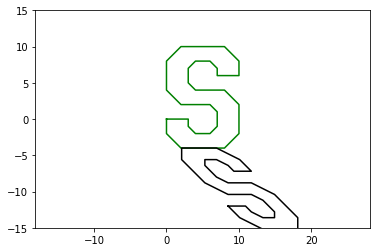
✅ **Questions:** What where the input values?
Put your answer here:
r =
scale =
dx =
dy =
shx =
shy =
In this section we are going to explore using transformations to generate fractals. Consider the following set of linear equations. Each one takes a 2D point as in put applies a $2 \times 2$ transform and then also translates by a $2 \times 1$ translation matrix
We want to write a program that use the above transformations to "randomly" generate an image. We start with a point at the origin (0,0) and then randomly pick one of the above transformation based on their probability, update the point position and then randomly pick another point. Each matrix adds a bit of rotation and translation with $T_4$ as a kind of restart.
To try to make our program a little easier, lets rewrite the above equations to make a system of "equivelent" equations of the form $Ax=b$ with only one matrix. We do this by adding an additional variable variable $z=1$. For example, verify that the following equation is the same as equation for $T1$ above:
$$ T_1: \left[ \begin{matrix} x_1 \\ y_1 \end{matrix} \right] = \left[ \begin{matrix} 0.86 & 0.03 & 0 \\ -0.03 & 0.86 & 1.5 \end{matrix} \right] \left[ \begin{matrix} x_0 \\ y_0 \\ 1 \end{matrix} \right] $$Please NOTE that we do not change the value for $z$, and it is always be $1$.
✅ **DO THIS:** Verify the $Ax=b$ format will generate the same answer as the $T1$ equation above.
The following is some pseudocode that we will be using to generate the Fractals:
- Let $x = 0$, $y = 0$, $z=1$
- Use a random generator to select one of the affine transformations $T_i$ according to the given probabilities.
- Let $(x',y') = T_i(x,y,z)$.
- Plot $(x', y')$
- Let $(x,y) = (x',y')$
- Repeat Steps 2, 3, 4, and 5 twenty thousand times.
The following python code implements the above pseudocode with only the $T1$ matrix:
%matplotlib inline

import numpy as np
import matplotlib.pylab as plt
import sympy as sym
sym.init_printing(use_unicode=True) # Trick to make matrixes look nice in jupyter

T1 = np.matrix([[0.86, 0.03, 0],[-0.03, 0.86, 1.5]])
#####Start your code here #####
T2 = T1
T3 = T1
T4 = T1
#####End of your code here#####

prob = [0.83,0.08,0.08,0.01]

I = np.matrix([[1,0,0],[0,1,0],[0,0,1]])

fig = plt.figure(figsize=[10,10])
p = np.matrix([[0.],[0],[1]])
plt.plot(p[0],p[1], 'go');
for i in range(1,1000):
    ticket = np.random.random();
    if (ticket < prob[0]):
        T = T1
    elif (ticket < sum(prob[0:2])):
        T = T2
    elif (ticket < sum(prob[0:3])):
        T = T3
    else:
        T = T4
    p[0:2,0] = T*p
    plt.plot(p[0],p[1], 'go');
plt.axis('scaled');

✅ **DO THIS:** Modify the above code to add in the $T2$, $T3$ and $T4$ transforms.
✅ **QUESTION:** Describe in words for the actions performed by $T_1$, $T_2$, $T_3$, and $T_4$.
$T_1$: Put your answer here
$T_2$: Put your answer here
$T_3$: Put your answer here
$T_4$: Put your answer here
✅ **DO THIS:** Using the same ideas to design and build your own fractal. You are welcome to get inspiration from the internet. Make sure you document where your inspiration comes from. Try to build something fun, unique and different. Show what you come up with with your instructors.
#Put your code here.
Congratulations, we're done!
If you attend class in-person then have one of the instructors check your notebook and sign you out before leaving class. If you are attending remote, turn in your assignment using D2L.
Course Resources:
Written by Dr. Dirk Colbry, Michigan State University

This work is licensed under a Creative Commons Attribution-NonCommercial 4.0 International License.