Day 14 Pre-Class Assignment: Fitting models, making predictions, and evaluating fits using data#
Goals for today’s assignment#
Describe the utility of fitting trendlines to data, in the context of making predictions about the future
Use best-fit lines to make predictions about future values
Quantitatively and qualitatively describe how to determine the Goodness of fit for a given line
Assignment instructions#
This assignment is due by 11:59 p.m. the day before class, and should be uploaded into the appropriate “Pre-class assignments” submission folder. If you run into issues with your code, make sure to use the Teams channel to help each other out and receive some assistance from the instructors. Submission instructions can be found at the end of the notebook.
1. Predicting Future Trends#
Consider the following dataset showing salinity of water (amount of salt in the water) versus depth for an imaginary body of water:
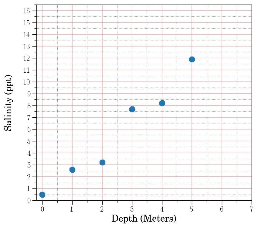
✅ 1.1 What would you guess the salinity would be at a depth of 6 meters? At 7 meters? What makes you think those would be the values?
✎ Put your answer here.
✅ 1.2 Now, make a line connecting the first and last points and continue it out to a depth of 7 meters. Using the line, predict what the salinity would be at a depth of 6 and 7 meters. You may find it useful to hold a straight edge up to your screen (e.g. piece of paper, pen, pencil) to trace out this line.
✎ Put your answer here.
✅ 1.3 How do the values you determined using your line compare with the values you predicted in 1.1?
✎ Put your answer here.
2. Determining the Line of Best Fit?#
Consider the figure below, which shows the same data set, but with two lines.
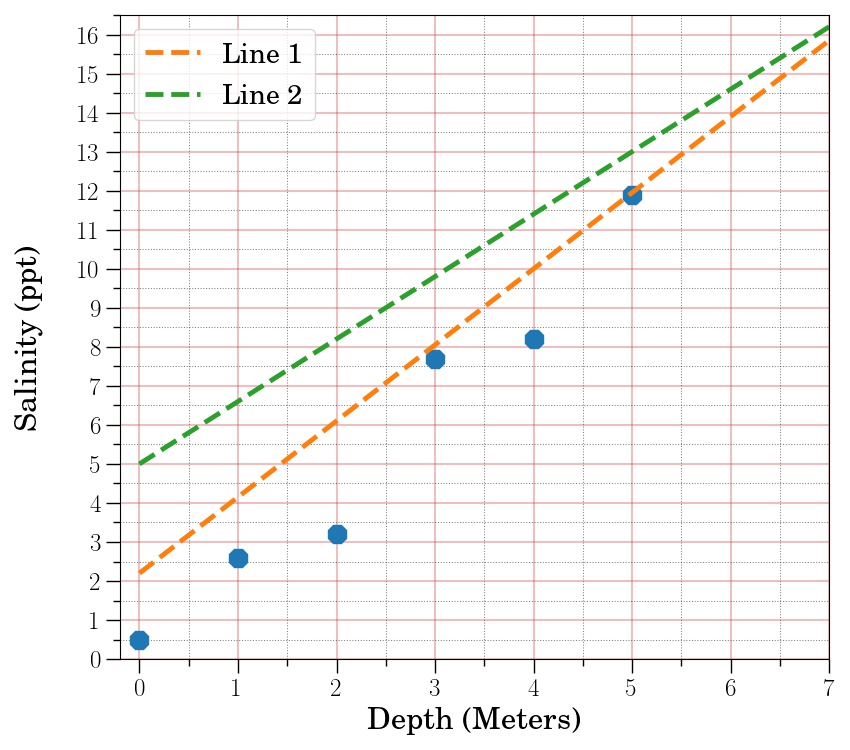
✅ 2.1 Without doing any calculations (i.e., just looking at the figure), do you think the salinity at a depths of 6 and 7 meters will be closer to values in line 1 or line 2? What is it about that particular line that makes you think it will be more accurate in predicting future values?
✎ Put your answer here.
✅ 2.2 Imagine someone asks you to show quantitatively that the line you have selected will be more accurate in predicting future values. What is a way you could quantitatively measure how well a line fits some dataset?
Try to come up with an algorithm–that is, a detailed procedure, like a recipe–for calculating how well a line fits a dataset.
✎ Put your answer here.
✅ 2.3 Now try to apply your algorithm (by hand) to the lines and data from the figure above. Does the line you choose in part 2.1 fit the data the best according to your algorithm?
The data values and the values for the two lines are provided.
import numpy as np

x_data = np.array([0,1,2,3,4,5])
y_data = np.array([0.5,2.6,3.2,7.7,8.2,11.9])
y_values_line_1 = np.array([2.2, 4.15, 6.1, 8.05, 10., 11.95, 13.9, 15.85])
y_values_line_2 = np.array([5., 6.6, 8.2, 9.8, 11.4, 13., 14.6, 16.2])
✎ Put your answer here.
3. Using a Computer to Fit a Line#
In the questions and exercises above, you were asked to think through how one might determine the “best fit” line that matches the data you were presented with. Using code, we can calculate such fits quantitatively both by writing code “from scratch” or by using built-in tools from pre-existing Pythong packages. One such pre-existing tool is called curve_fit which is part of the Python package SciPy. The curve_fit function can be used to fit a mathematical model to data. We’ll be using this in class, so it’s important that you spend some more time trying to get a better idea of how it works.
Note: By “fitting a function”, we mean that there is a function that contains parameters that we can adjust to find the expected values that fit the data the best (hence finding the “best fit”).
To use curve_fit, you need a minimum of two things:
A (Python) function that contains the mathematical function you are fitting to your data
A dataset, consisting of x and y values, that you are fitting your mathematical function to.
Let’s look at an example.
Below is a set of x and y values, and we want to fit the following function:
✅ 3.1 What parameters are we adjusting to find the best fit for this function?
✎ Put your answer here.
Generating some data to demonstrate the process of fitting a model to data#
The cell below create two arrays of data, a set of x values and a set of y values. The x values are the independent variable and the y values are the dependent variable. We’ll use these as our test data for fitting the function from above.
import numpy as np
import matplotlib.pyplot as plt
%matplotlib inline

x = np.array([0.00, 0.71, 1.43, 2.14, 2.86, 3.57, 4.28, 5.00, 5.71, 6.43, 7.14, 7.85])
y = np.array([0.34, 1.42, 1.92, 1.23, -0.08, -1.19, -0.82, -0.14, 0.90, 1.77, 1.78, 0.30])

plt.plot(x,y)
Fitting our model#
To get started with finding our fit, we first define a Python function that contains the mathematical function we’re fitting.
def sin_function(x, A, B, C):
    return A * np.sin(B * x + C)
We now have the two pieces needed to use curve_fit, (1) the function we’re using and (2) the data we’re trying to fit, so let’s run it and see what we get.
from scipy.optimize import curve_fit

best_fit_parameters, just_ignore_this_for_now = curve_fit(sin_function, x, y)
print(best_fit_parameters)
If we look at the documentation for curve_fit, we see that by this calling function, we get two return values by default: popt and pcov. popt contains the best fit parameters. You do not need to worry about pcov for the purposes of this assignment, but you are encouraged to read the documentation for a description of what pcov is.
In the code above, popt was stored in the best_fit_parameters variable, and pcov was stored in just_ignore_this_for_now.
If we want to see what our best fit line looks like using our best fit parameters, we can use the following code:
A_expected = best_fit_parameters[0]
B_expected = best_fit_parameters[1]
C_expected = best_fit_parameters[2]

y_expected = sin_function(x, A_expected, B_expected, C_expected)
✅ 3.2 Give a brief explanation for what the last line of code is doing in the cell above.
✎ Put your answer here.
Now we can try to plot both the data and our best fit model values.
plt.scatter(x, y, label = "data")
plt.plot(x, y_expected, color = "orange", label = "fit")
plt.legend()
YOUR TURN#
One of the simplest functions you can have is a straight line, which takes the form:
✅ 3.3 What parameters would we adjust to find the best fit for this function?
✎ Put your answer here.
✅ 3.4 Fit a straight line to the x and y dataset provided below. Specify what the best fit parameters are and make a plot showing your best fit line. Remember, in order to use curve_fit to find the best-fit line, you’ll need to define a new function that match the mathematical function for the line, shown above. You should be able to use the code from above for the sine curve data as a guide for how to set everything up.
x = np.array([0,1,2,3,4,5])
y = np.array([0.5,2.6,3.2,7.7,8.2,11.9])

#Put your code here
4. Determining Goodness of Fit#
✅ 4.1 Compare your the best fit line you just found to the “best fit” line provided in Section 2. Which one appears to fit the data better?
✎ Put your answer here.
✅ 4.2 Try to turn the algorithm you described in part 2.2 for measuring how well a line fits the data into code and apply it to the new best fit line that you just found using curve_fit. How does this value for goodness of fit compare to the one you found in part 2.3?
#Put your code here
✎ Put your answer here.
Assignment wrap-up#
Please fill out the form that appears when you run the code below. You must completely fill this out in order to receive credit for the assignment!
from IPython.display import HTML
HTML(
"""
<iframe
	src="https://forms.office.com/r/r6xc6jHPg8"
	width="800px"
	height="600px"
	frameborder="0"
	marginheight="0"
	marginwidth="0">
	Loading...
</iframe>
"""
)
Congratulations, you’re done!#
Submit this assignment by uploading it to the course Desire2Learn web page. Go to the “Pre-class assignments” folder, find the appropriate submission link, and upload it there.
See you in class!
© Copyright 2024, The Department of Computational Mathematics, Science and Engineering at Michigan State University