Homework 3: Loading, Cleaning, Analyzing, and Visualizing Data with Pandas (and using resources!).#
Exploring Nahuatl names of plants and ahuacatl (avocado) production#
✅ Put your name here
#
Learning Goals#
Using pandas to work with data and clean it
Make meaningful visual representations of the data
Fitting curves to data and evaluating model fits
Assignment instructions#
Work through the following assignment, making sure to follow all of the directions and answer all of the questions.
If you struggle to load data files, try downloading the homework assignment and CSV file. Then complete it in Jupyter and upload your completed files to CodeGrade at the end.
Grading#
(0) Academic Integrity (2 pts)
(1) Reading, Describing, and Cleaning Data (22 pts)
(2) Exploratory Data Analysis (25 pts)
(3) Fitting Curves to Data (24 pts)Total points possible: 73
Part 0. Academic integrity statement (2 points)#
In the markdown cell below, paste your personal academic integrity statement. By including this statement, you are confirming that you are submitting this as your own work and not that of someone else.
✎ Put your personal academic integrity statement here.
Before we read in the data and begin working with it, let’s import the libraries that we would typically use for this task. You can always come back to this cell and import additional libraries that you need.
import pandas as pd
import matplotlib.pyplot as plt
import numpy as np
import math
from scipy.optimize import curve_fit
Part 1: Reading, describing, and cleaning data (22 total points)#
Mexico recognizes 63 indigenous languages. By far, the largest of these languages is Nahuatl, with over 1.6 million speakers in Mexico. The name “Mexico” itself is derived from the mexica people, who established Tehochtitlan which is now Mexico City. Nahuatl and related languages are spoken throughout Mexico and spread all the way north into what is now the United States of America and all the way south to Central America.
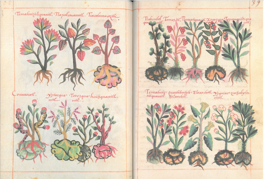
It is not surprising that domesticated plants from Mexico retain their names in Nahuatl, and that these names–and the cultural uses of the plants–have spread globally. For example, Nahuatl words like chÄ«lli (chile), cacaotl (chocolate), tomatl (tomato), and Ähuacatl (avocado) have been incorporated into langauges around the world, just as the uses of these plants have been globally incorporated as well. Remarkably, we have a record of both Nahuatl names for plants and illustrations of them. The De la Cruz-Badiano Codex of 1552, written shortly after Conquest, was written by a Nahuatl physician (tÄ«citl), and demonstrated the medicinal value of plants Nahua people used, as well as documenting botanical details about plants in Mexico. We have been studying the De la Cruz-Badiano codex and recently wrote a manuscript applying data science techniques to analyze the Nahuatl names, text, and botanical illustrations in it. We also created a website that you can browse the text and illustrations in this manuscript.
In the first part of the assignment, you will use the provided dataset
nahuatl_names.csvto explore the Nahua classification of plants into 5 major groups:
xihuitl(“herb or leaf or green”)
quahuitl(“tree or woody”)
xochitl(“flower”)
patli(“medicine or remedy”)
quilitl(“edible green”)
1.1 Read the data (1 point)#
✅ Task
Read in the data from
nahuatl_names.csvinto a Pandas dataframe.Display the
headof the data.
## your code here
1.2 Describe the data (3 points)#
1.2.1 ✅ Task (1 point)#
Use
describeto display several summary statistics from the data frame.
## your code here
1.2.2 ✅ Task (2 points)#
Using the results from
describein 1.2, answer the following questions:
Relative to the total number of entries in
nahuatl_name, how many entries are present in thetypeandclasscolumns?How do you explain the discrepancy between the count of the
typeandclasscolumns Hint: refer to the results of usingheadon the df from the question above. Beyond the classes listed above, what else do you see?
✎ Put your answers here:
1.3 Isolating and performing basic statistics on data (4 points)#
1.3.1 ✅ Task (1 point)#
Display the
typecolumn on its own using the name of the column.
## your code here
1.3.2 ✅ Task (1 points)#
Using
.iloc, display the first five rows of just thetypecolumn.
## your code here
1.3.3 ✅ Task (2 points)#
Using
value_countsandmodefunctions, print out the count of each level oftypeand the most abundant level, respectively.Note: we don’t typically think of using
modeon categorical data, but just like continuous data, it represents the most prevalent class. Also note that the De la Cruz-Badiano is a codex/herbal mostly about plants
## your code here
1.4 Filter the data using masking (10 points)#
1.4.1 ✅ Task (5 points)
For each of the six plant classes in
class, you want to know how many entries are represented.
For each of the six classes below, calculate the total number of entries using masking.
xihuitl(“herb or leaf or green”)
quahuitl(“tree or woody”)
xochitl(“flower”)
patli(“medicine or remedy”)
quilitl(“edible green”)
multiple(there are multiple classes of the above five represented in the name)Print your results for each of six class levels. From your mask, the function
.sum()can be used to find the count of each class.Your results should look like:
The count of class xihuitl is X
The count of class quahuitl is X
The count of class xochitl is X
The count of class patli is X
The count of class quilitl is X
The count of class multiple is X
## your code here
1.4.2 ✅ Task (5 pts)
One of the classes of
classismultiple, in which multiple plant classes are represented.
Using masking, display or print out the entries in
nahuatl_namethat belong to themultipleclass inclass.From the entries that you printed out, choose one name. Write that name out and write at least two of the plant class names that you see within it. Note: Within a name,
xihuitlcan be represented asxiuh-andquahuitlasquauh-orquauhtla.
# your code here printing out "nahuatl_name" of entries of "multiple" class (3 pts)
Answer the following questions:
What Nahuatl name did you choose?
Which plant classes do you see in the name?
✎ Put your answer here.
1.5 Clean out the NaN values (4 points)#
1.5.1 ✅ Task (2 points)#
There are so many
NaNvalues in theclasscolumn! Create a new, “clean” dataframe calledclean_nahuatl_dfthat removes any entry withNaNvalues. Use the built in pandas functiondropnato do this (google it to learn more!).
## your code here
1.5.2 ✅ Task (2 points)#
Now that you have the original and clean datasets:
Determine the number of rows in each of them.
Print out your results.
## your code here
Part 2: Exploratory Data Analysis (21 total points)#
One of the most popular Nahuatl-named plants in recent years is avocado, en español aguacate and in Nahuatl Ähuacatl. You think to yourself that to accomodate the global demand of guacamole (in Nahuatl ÄhuacamÅlli) that surely Mexico must be producing a lot more avocados in recent years! In fact, you wonder what other countries are the top avocado produces, and find Colombia and Dominican Republic just after Mexico.
A rich resource for the statistics of global agricultural production of most crops is the statistical service of the Food and Agriculture Organization of the United Nations (FAOSTAT). There, you find data relating to avocados in these three countries from 1961 to 2024.
The avocado data is provided to you as the
ahuacatl.csvdataset.It’s time to explore the data! Let’s visualize our data and look for correlations in our ahuacatl dataset.
Part 2.1: Correlations (5 points)#
From 1961 to 2024, we have the avocados produced in tonnes for three countries in the columns
mexico,colombia, anddominican_republic.✅ Do this:
Read in the file
ahuacatl.csvas a dataframePrint or display a correlation matrix between the values in the columns of
mexico,colombia, anddominican_republic.Hint 1: Look up the pandas
corrfunction for dataframes.
Hint 2: To select multiple columns, use the following notation:df[["col1"], ["col2"]]
# Put your code here
✅ Answer this question:
In your opinion, would you consider any of the correlations between the columns to be strong?
What direction are the correlations, positive or negative?
In your own words, describe what you believe the correlations demonstrate for avocado production between the three countries?
✎ Put your answers here.
Part 2.2: Visualizing the data (16 points)#
The numbers above gives us a quantitative measure of the correlations in the dataset. But we need to see the data! Visualization in data science is a very important skill.
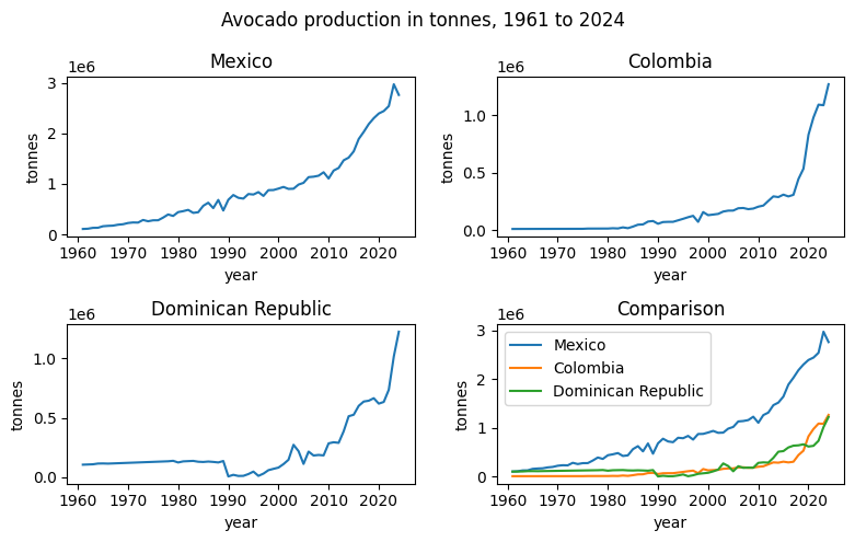
In the next exercise, you will visualize the relationships between these variables as scatterplots. You will create a plot for each relationship: 1)
mexicovs.year, 2)colombiavs.year, 3)dominican_republicvs.year, and 4) plots ofmexico,colombia, anddominican_republictogether vs.year.In the end, your plot should look similar to the one below:
✅ Do this (13 points):
Create 4 subplots using
plt.subplot. Use 2 rows and 2 columns (4 points).Use
plt.figureand the argumentfigsizeto make a plot 8 inches wide x 5 inches long (1 point).Plot 1)
mexicovs.year, 2)colombiavs.year, 3)dominican_republicvs.year, and 4)mexico,colombia, anddominican_republictogether vs. year (1 point).Provide a title for each subplot as follows:
Mexico,Colombia,Dominican Republic, andComparison(1 point).Give the overall plot the title
Avocado production in tonnes, 1961 to 2024(1 point)Provide x-axis labels as
year(1 point).Provide y-axis labels as
tonnes(1 point).For the final
Comparisonplot, use thelabelargument for each country and create a legend (2 points).Use
tight_layoutto give your plot optimal sizing (1 points).
# Put your code here
✅ By examining the plots you’ve created, answer the following questions (3 points):
How can the plots help explain the correlation coefficients you calculated in the previous question?
Which country is producing the most avocados overall?
Are there any interesting patterns you see in production over time for any country? What are they?
✎ Put your answers here.
Part 3: Fitting curves to data. Harvest date as a function of temperature anomaly (20 points)#
Now that we have visualized our data we can formulate a question in a guided way. In this section, we will ask:
What is the relationship between year and avocado production in Mexico? Can we predict avocado production by year and into the future?
Part 3.1: Model (4 points)#
In the above plots you created for 2.2, notice that production in tonnes (
mexico) exponentially increases in value asyearincreases. Specifically,\[production(t) = a e^{b t} + c\]Where \(production\) is the production of avocados in tonnes for Mexico represented by the column
mexico, and \(t\) is the time in years represented by the columnyear.
a,b, andcare parameters to be modeled that represent the following:
ais the initial scale (how much production âtakes offâ)
bis the growth rate (the star of the show)
cis the baseline offset (prevents forcing the curve through zero)✅ Do the following:
Write a function calledexp_growththat calculates \(production\) based on \(t\) in years using the equation above. The equation should be constructed so that you can build a model using thecurve_fitfunction in the next section.
# Put your code here
Part 3.2: Fit the model (8 points)#
✅ Do the following:
For the time variable
t, you need to subtract 1961. This is because the data starts on year 1961 and we need to start at 0 for the model to be fit (1 point)To fit your model successfully, you must use the suggested initial parameter values argument
p0withcurve_fitthat was discussed in class. You should use the followingp0argument to fit your model successully (1 point):p0 = [2e6, 0.04, 1e5]Now use
curve_fitwith yourexp_growthfunction to find the \(a\), \(b\), and \(c\) parameters. (3 points)Print out the value of \(a\), write “The value of a is…” (1 point)
Print out the value of \(b\), write “The value of b is…” (1 point)
Print out the value of \(c\), write “The value of c is…” (1 point)
# Put your code here
Part 3.3 Check your model (8 points)#
✅ Do this (6 points): Make a plot comparing your model and the data.
Plot the actual data (2 points)
Plot your modeled data (2 points)
Use x and y axis labels and title (1 point)
Remember to substract 1961 from the year to zero out the time variable! (1 point)
# Put your code here
✅ Answer the following questions (2 points):
Do you think your model is a good model for the years represented in the data?
Do you think your model we accurately predict avocado production in Mexico in the future? Clearly justify your answer (looking for more than a “yes” or “no” answer).
✎ Put your answers here.
Congratulations, you’re done!#
© 2024 Copyright the Department of Computational Mathematics, Science and Engineering.