Homework 4: Compartmental Models + Data Visualization (SPRING 2026)#
Assignment instructions#
Work through the following assignment, making sure to follow all of the directions and answer all of the questions.
This assignment is due at 11:59pm on Friday, April 10th, 2026
It should be uploaded into D2L Homework #4. Submission instructions can be found at the end of the notebook.
Table of Contents#
Part 0. Academic Integrity Statement (2 points)
Part 1. Understanding compartmental models (20 points)
Part 2. Simulating differential equations (20 points)
Part 3. Interpreting results of simulations (15 points)
Part 4. Data visualization (20 points)
Part 5. Data interpretation (16 points)
Total points = 93.
Part 0. Academic integrity statement (2 points)#
In the markdown cell below, paste your personal academic integrity statement. By including this statement, you are confirming that you are submitting this as your own work and not that of someone else.
✎ Put your personal academic integrity statement here.
Part 1. Understanding compartmental models (20 total points)#
Malaria is caused by a parasite called Plasmodium falciparum, that undergoes several transformations during the lifecycle. After its initial form, sporozoites, penetrates the blood stream (thourgh a mosquito bite), it populates the liver where it produces the blood-stage called merozoites. Merozoites populate the red blood cells, and this is what causes the malaria symptoms. In this form however, the parasite is not transmissble. For transmission, another, non-replicating form, called gametocyte may develop through conversion from merozoites. The infection triggers response of immune effectors (i.e. white blood cells).
While the process is complicated, some general features may be learned through compartmental modeling. Examine the compartmental model diagram below.
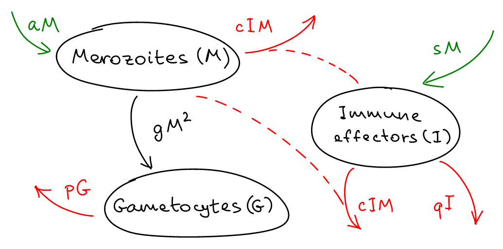
✅ Part 1.1 (4 points)
Describe in the cell below: how many compartments there are in the model, and what each of the compartments stands for.
✎ Put your answer here
✅ Part 1.2 (8 points)
For each of the pathways or arrows in the model, give an interpretation for what actual process might be represented.
✎ Put your answer here
✅ Part 1.3 (8 points)
In the cell below, write down the ordinary differential equations associated with this compartmental model.
✎ Put your answer here
Part 2. Solving differential equations numerically (20 total points)#
In previous assignments, you have used solve_ivp to compute the numeric solution of the logistic model of the growth of a single population. Recall, the Logistic population model is described by the following differential equations:
\begin{equation} \frac{dP}{dt} = kP\Big(1-\frac{P}{C}\Big), \end{equation}
where \(P =\) population, \(k =\) growth rate, and \(C =\) the carrying capacity.
Examples code for computing the solution for for \(P_0 =0.1\) billion (initial population), \(k=1\), and \(C =1\) billion is provided below:
# example code to compute a numeric solution of the logistic model
import numpy as np
from scipy.integrate import solve_ivp

# define the derivative
def logistic(time, current_state):
    p = current_state
    dpdt = p*(1-p)
    return dpdt

# compute numeric solution
initial_p = [0.1]
time = np.linspace(0,10,50)

result = solve_ivp(logistic, (0,20), initial_p, t_eval = time)

# unpack solution
numerical_p = result.y[0,:]
The above was a logistic model for a single species. Now let’s consider a two-variable system, represented by two coupled (linked) differential equations.
A classic example of a two-variable system is a bead on a rotating hoop. Imagine a circular wire hoop standing vertically that is spinning at a constant angular velocity v around its vertical diameter. A small, frictionless bead is threaded onto the hoop. As the hoop spins, two main forces act on the bead: gravity (pulling it down) and centrifugal force (pushing it outward away from the axis of rotation). Depending on how fast the hoop spins, the bead will either settle at the very bottom or “climb” up the side of the hoop to a specific angle.
To describe this system, we use the angle a (the position of the bead relative to the bottom) and its angular velocity (v). The dynamics are defined by the following two first-order differential equations:
(The rate of change of the angle a is the angular velocity v.)
(The rate of change of the angular velocity v depends on the balance between centrifugal force and gravity, where g is gravity and r is the hoop’s radius.)
Your job for this part of the assignment is implementing and computing the numeric solutions for the two-variable bead on a rotating hoop model as described by the two equations above. You can do so by adapting the code for the logistic model above.
✅ Part 2.1 (8 points)
Define the derivatives function for the two-variable bead on a rotating hoop model in the cell below (to be used as an input later for solve_ivp – so pay attention to the format).
The function should take in the time, a current-state vector containing the angle a and the angular velocity v, and return the derivatives of the angle and angular velocity. It will also take in the parameters g and r for the gravity and the radius of the hoop, respectively.
# write your function here
✅ Part 2.2 (6 points)
Using solve_ivp, compute the numeric solution for two rotating-hoop model with:
the parameters Gravity \(g = 9.81\) (\(m/s^2\)), and radius of the hoop \(r=1.0\) (\(m\)),
initial conditions \([a_0,v_0]= [0.1, 0.0]\),
the final time = \(20\) (\(s\)).
Unpack the result you get from solve_ivp into separate variables a and v.
# put your code here
✅ Part 2.3 (4 points)
Plot the solutions of \(a\) and \(v\) as a function of time in the cell below. Be sure to add appropriate axis labels and legends, and a plot title.
# put our code here
✅ Part 2.4 (2 points)
What happens when you run the model longer? Does the pattern of time evolution change for either \(a(t)\) or \(v(t)\)?
✎ Put your answer here
Part 3. Interpreting model behavior for different parameters and initial conditions (15 total points)#
In part 2, the parameter values you were given generated the “Subcritical Regime” where the bead oscillated back and forth. (\(w < \sqrt{g/R}\))
In this part, you will re-run the model under a couple of different scenarios and initial conditions, and interpret these plots.
✅ Part 3.1 (4 points) Supercritical Regime
Let us pick a value of \(w\) that is greater than \(\sqrt{g/R}\), and re-run the model.
Rerun your code from part 2.2 and regenerate the plots from part 2.3, but this time let \(w = 3.5\).
# Put your code to call `solve_ivp` here
# Put your code to plot the solution here
✅ Part 3.2 (3.5 points) How did the behavior of the system change? Do you still see oscillations in \(a(t)\) and \(v(t)\)?
✎ Put your answer here
✅ Part 3.3 (4 points) High-Speed Limit
Let us now pick a value of \(w\) that is much greater than \(\sqrt{g/R}\), and re-run the model.
Rerun your code from parts 2.2 and 2.3, but this time let \(w = 6\).
# Put your code to call `solve_ivp` here
# Put your code to plot the solution here
✅ Part 3.4 (3.5 points) How did the behavior of the system change this time? Do you still see oscillations in \(a(t)\) and \(v(t)\)?
✎ Put your answer here
Part 4. Data Visualization for NYC’s “Vision Zero” Initiative#
In 2014, New York City launched Vision Zero, an ambitious plan to eliminate all traffic-related fatalities and serious injuries. The city has significantly invested in “traffic calming” measures, lower speed limits, and thousands of automated speed cameras. However, the path to zero has been bumpy.
You have been tasked with analyzing the raw NYPD collision data to see if the streets of New York are actually getting safer, or if the “Vision Zero” goal remains elusive.
✅ Part 4.1 (4 points) Data Context
You found the collision data on the NYC Open Data portal. Briefly contextualize the data in the cell below by answering the following:
Who collected/generated the data?
How was the data collected/generated?
Who/what is included in the data?
What are the limitations or biases of the data?
✎ Put your answer here
✅ Part 4.2 (4 points) Loading and cleaning data
Now that you know the context of the data, it’s time to read it into your notebook and prepare it for analysis. Because the original dataset is massive (over 2 million rows), we are working with a sampled subset of 5,000 crashes. However, this sample is still “raw” and requires cleaning.
In the cell below:
Read in the data file
nypd_collisions_sample.csv.Remove any rows where ‘BOROUGH’ is NaN and save this as a new dataframe.
Drop the columns ‘CONTRIBUTING FACTOR VEHICLE 3’, ‘CONTRIBUTING FACTOR VEHICLE 4’, and ‘CONTRIBUTING FACTOR VEHICLE 5’ from your new dataframe.
Display the
.shape,and the.head()of your cleaned dataframe.
If your cleaning worked correctly, you should have roughly 3,500 rows and 19 columns remaining.
# put your code here
✅ Part 4.3 (4 points) Choosing a question and getting the data
Recall the key pieces to an effective data visualization (from the Day 20 Pre Class and In Class assignments). There are many ways to look at this crash data to see if NYC’s “Vision Zero” goals are being met. For this section, you will choose one of the following Research Questions (RQ) to explore:
RQ 1: How does the total number of persons injured compare across the five boroughs for the most recent complete year in our data (2025)?
RQ 2: Compare the number of “Pedestrians Injured” vs. “Cyclists Injured” for each borough. Which borough appears to have the highest “non-motorist” injury count in this sample?
RQ 3: Choose one specific borough (e.g., Brooklyn, Manhattan, etc.). How has the total number of injuries changed year-over-year from 2014 to 2025?
In the cells below:
Indicate which question you are going to explore.
Using your clean data set, extract the data necessary for answering your question (i.e., use masking to extract data, remove rows or columns you will not use, etc.).
Display the first few rows of your extracted data subset.
✎ Write down your choice and specify the variables involved.
# put your code here to extract a subset of data relevant to your question
✅ Part 4.4 (8 points) Making a Plot
Now that you have extracted the specific data you need, it’s time to create a visualization! Using the plotting tools we have explored in class (matplotlib.pyplot or seaborn), create a plot that answers your chosen Research Question.
Your plot will be graded based on the following rubric:
Does the plot tell a story? (4 Points): Is it clear what the data is showing and how it answers your RQ?
Chart type (2 points): The chart type is appropriate, and the data is easy to read.
Labels, legend, and title (1 point): Are they informative without being cluttered?
Presenting multi-variable data (1 point): Did you effectively use colors, markers, or grouping to show different categories?
# put your code here to create a plot
Part 5. Data Interpretation#
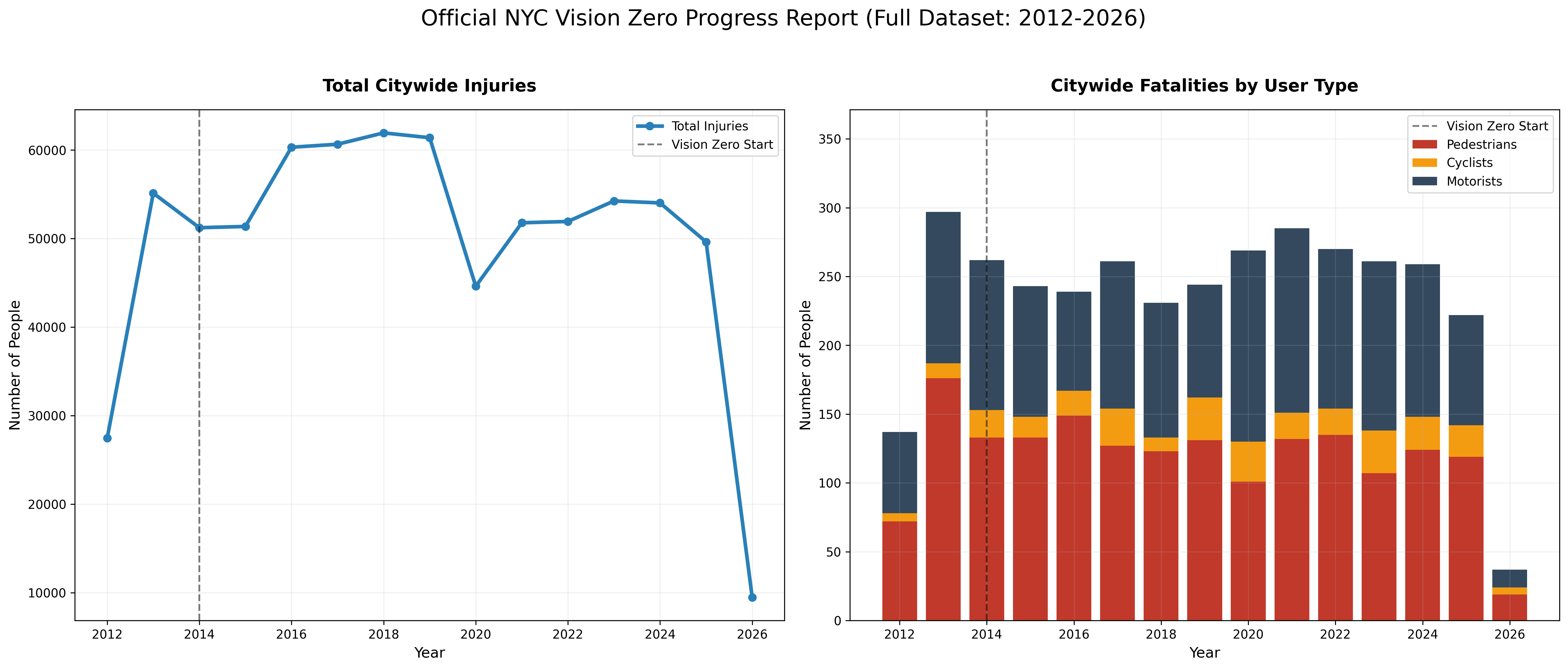
Now that you have explored your own subset of the data, it is time to look at the “Big Picture.” Below are some figures generated using the full dataset of over 2.2 million records.
In this final section, you will step into the shoes of an NYC Policy Analyst working on the Vision Zero initiative.
✅ Part 5.1 (6 points) Data Artifacts
Analyze the plots below and answer the following questions.
1. The 2012 “Rise” (2 points): In both plots there is a massive jump between 2012 and 2013. What might be the cause of that?
2. The 2026 “Cliff” (2 points): What explains the dramatic drop-off that both plots show in 2026?
2. Progress (2 points): From these plots, do you think the Vision Zero initiative has been successful?
✎ Put your answer here
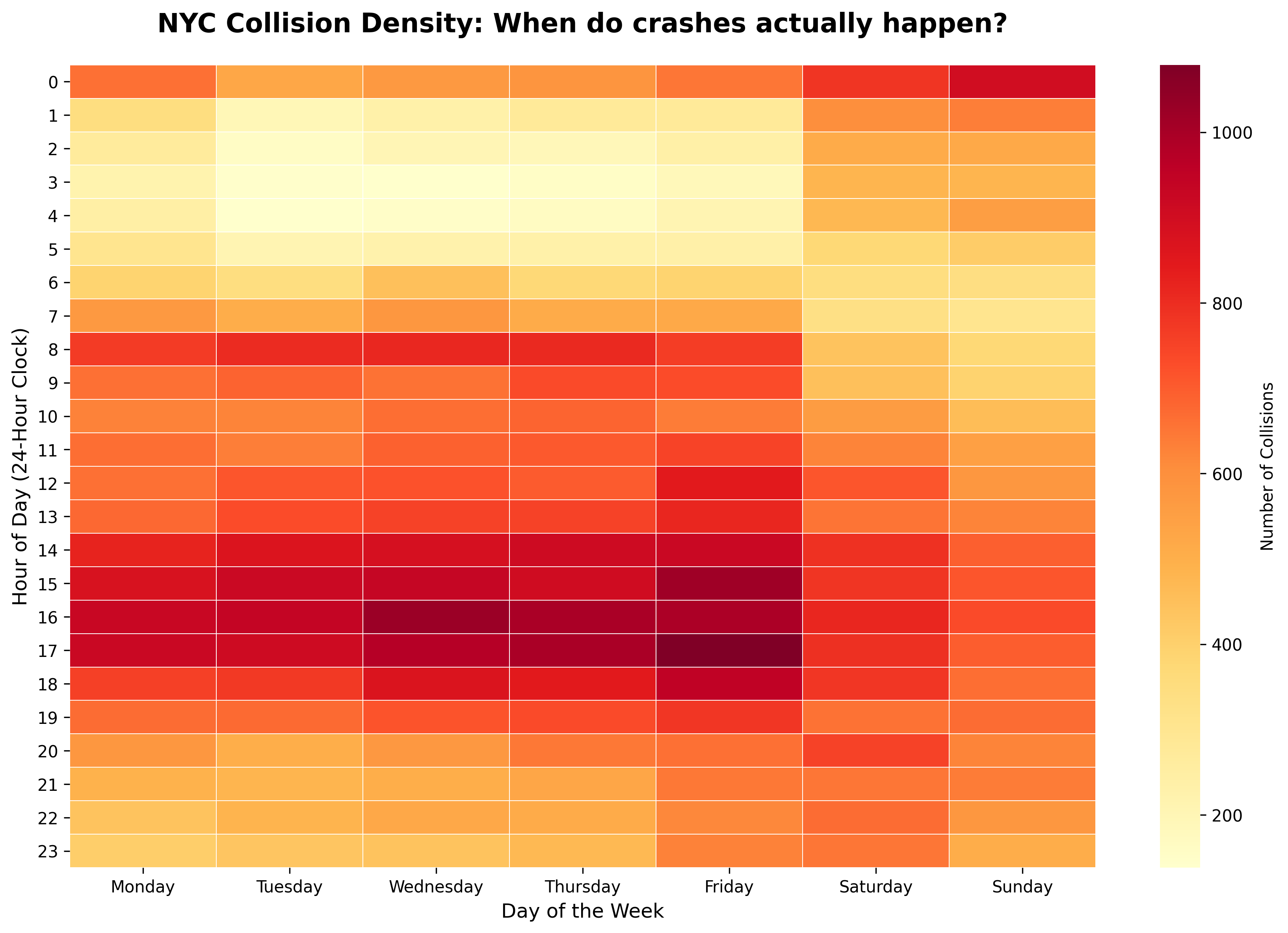
✅ Part 5.2 (4 points) When do crashes occur?
To truly understand traffic safety, we must also investigate when they occur. The following heatmap provides a look at a typical week.
1. Dangerous Hours (2 points) What seem to be some of the most dangerous times of day? Why do you think that is?
2. Policy & Prevention (2 points) If a “Vision Zero” task force could only implement one safety intervention for four hours a week, which specific blocks on this heatmap should they target to have the greatest impact?
✎Put your answer here
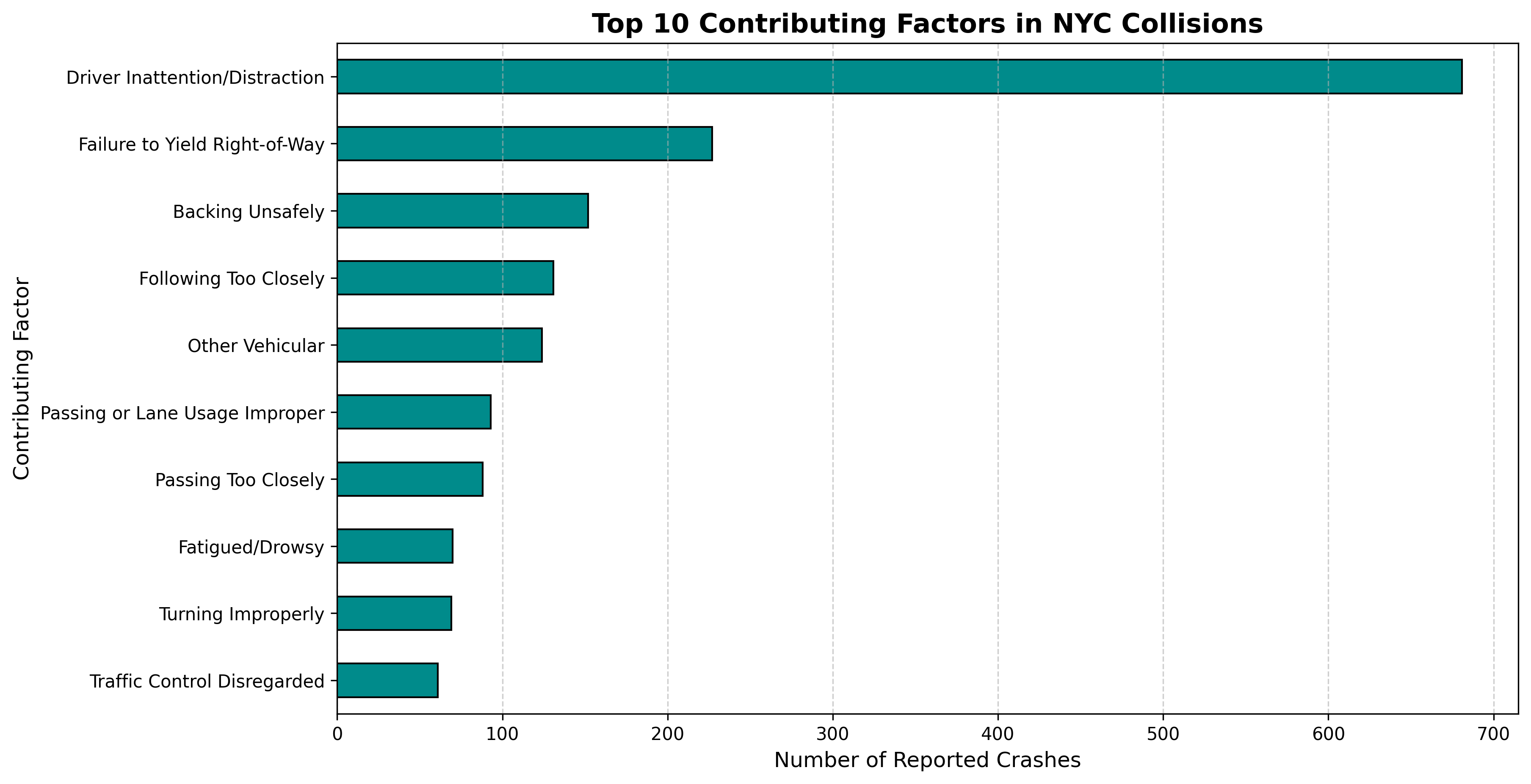
✅ Part 5.3 (6 points) Why do crashes occur?
To reach the goal of “Zero,” we must also understand the cause. The visualization below explores the “Why.” By ranking the primary contributing factors reported by the NYPD, we can identify whether the biggest threats to New Yorkers are rooted in road infrastructure or individual driver behavior.
1. Policy Intervention (2 point) If the top factor is “Driver Inattention/Distraction,” would building more bike lanes solve this specific problem? Why or why not? What kind of policy (e.g., laws, technology, or education) might be more effective?
2. The “Unspecified” Gap (2 point) In our code, we manually removed the “Unspecified” category. If “Unspecified” were actually the largest category in the dataset, how would that make the job of a safety analyst more difficult?
3. Vision Zero Goal (2 point) Looking at these 10 factors, which one do you think is the hardest for the city to eliminate to reach their goal of zero traffic deaths? Justify your choice.
✎ Put your answer here
Congratulations, you’re done!#
Submit this assignment by uploading your notebook to the course Desire2Learn web page. Go to the “Homework” folder, find the appropriate submission link, and upload everything there. Make sure your name is on it!
© Copyright 2026, Department of Computational Mathematics, Science and Engineering at Michigan State University